Chemistry 444
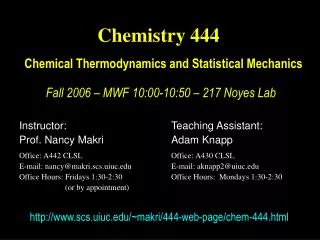
Chemistry 444. Chemical Thermodynamics and Statistical Mechanics. Fall 2006 – MWF 10:00-10:50 – 217 Noyes Lab. Instructor: Prof. Nancy Makri Office: A442 CLSL E-mail: nancy@makri.scs.uiuc.edu Office Hours: Fridays 1:30-2:30 (or by appointment).

Chemistry 444
E N D
Presentation Transcript
Chemistry 444 Chemical Thermodynamics and Statistical Mechanics Fall 2006 – MWF 10:00-10:50 – 217 Noyes Lab Instructor: Prof. Nancy Makri Office: A442 CLSL E-mail: nancy@makri.scs.uiuc.edu Office Hours: Fridays 1:30-2:30 (or by appointment) Teaching Assistant: Adam Knapp Office: A430 CLSL E-mail: aknapp2@uiuc.edu Office Hours: Mondays 1:30-2:30 http://www.scs.uiuc.edu/~makri/444-web-page/chem-444.html
Why Thermodynamics? • The macroscopic description of a system of ~1023 particles may involve only a few variables! “Simple systems”: Macroscopically homogeneous, isotropic, uncharged, large enough that surface effects can be neglected, not acted upon by electric, magnetic, or gravitational fields. • Only those few particular combinations of atomic coordinates that are essentially time-independent are macroscopically observable. Such quantities are the energy, momentum, angular momentum, etc. • There are “thermodynamic” variables in addition to the standard “mechanical” variables.
Thermodynamic Equilibrium In all systems there is a tendency to evolve toward states whose properties are determined by intrinsic factors and not by previously applied external influences. Such simple states are, by definition, time-independent. They are called equilibrium states. Thermodynamics describes these simple static equilibrium states. Postulate: There exist particular states (called equilibrium states) of simple systems that, macroscopically, are characterized completely by the internal energy U, the volume V, and the mole numbers N1, …, Nr of the chemical components.
The central problem of thermodynamics is the determination of the equilibrium state that is eventually attained after the removal of internal constraints in a closed, composite system. • Laws of Thermodynamics
What is Statistical Mechanics? • Link macroscopic behavior to atomic/molecular properties • Calculate thermodynamic properties from “first principles” (Uses results for energy levels etc. obtained from quantum mechanical calculations.)
The Course • Discovery of fundamental physical laws and concepts • An exercise in logic (description of intricate phenomena from first principles) • An explanation of macroscopic concepts from our everyday experience as they arise from the simple quantum mechanics of atoms and molecules. …not collection of facts and equations!!!
The Course Prerequisites • Tools from elementary calculus • Basic quantum mechanical results Resources • “Physical Chemistry: A Molecular Approach”, by D. A. McQuarrie and J. D. Simon, University Science Books 1997 • Lectures • (principles, procedures, interpretation, tricks, insight) • Homework problems and solutions • Course web site (links to notes, course planner)
Course Planner • Organized in units. • Material covered in lectures. What to focus on or review. • What to study from the book. • Homework assignments. • Questions for further thinking. http://www.scs.uiuc.edu/~makri/444-web-page/chem-444.html/444-course-planner.html
Grading Policy Homework 30% (Generally, weekly assignment) Hour Exam #1 15% (September 29th) Hour Exam #2 15% (November 3rd) Final Exam 40% (December 14th) Please turn in homework on time! May discuss, but do not copy solutions from any source! 10% penalty for late homework. No credit after solutions have been posted, except in serious situations.
Math Review • Partial derivatives • Ordinary integrals • Taylor series • Differential forms
f df x dx Differential of a Function of One Variable
Differential of a Function of Two Variables f f (x0, y0) y (x0, y0+dy) (x0, y0) (x0+dx, y0+dy) (x0+dx, y0) x
The Ideal Gas Law Extensive vs. intensive properties Units of pressure Units of temperature Triple point of water occurs at 273.16 K (0.01oC)
Deviations from Ideal Gas Behavior T=300K “compressibility factor” Ideal gas: z = 1 z < 1: attractive intermolecular forces dominate z > 1: repulsive intermolecular forces dominate
Van der Waals equation At fixed P and T, V is the solution of a cubic equation. There may be one or three real-valued solutions. The set of parameters Pc, Vc, Tc for which the number of solutions changes from one to three, is called the critical point. The van der Waals equation has an inflection point at Tc.
Isotherms (P vs. V at constant T) • Large V: ideal gas behavior. • Only one phase above Tc. • Unstable region: liquid+gas coexistence.
The law of corresponding states All gases behave the same way under similar conditions relative to their critical point. (This is approximately true.)
Virial Coefficients Using partition functions, one can show that
Simple Models for Intermolecular Interactions (a) Hard Sphere Model (b) Square Well Potential
Interpretation of van der Waals Parameters From the van der Waals equation, … Comparing to the result of the square well model, Comparing to the result of the hard sphere model with r-6 attraction,
The Lennard-Jones Model Attractive term: dipole-dipole, or dipole-induced dipole, or induced dipole-induced dipole (London dispersion) interactions.
Origin of Intermolecular Forces Only Coulomb-type terms! The Born-Oppenheimer Approximation: Electrons move much faster than nuclei. Fixing the nuclear positions, Adiabatic or electronic or Born-Oppenheimer states Electronic energies; form potential energy surface. Responsible for intra/intermolecular forces.
INTRODUCTION TO STATISTICAL MECHANICS The concept of statistical ensembles An ensemble is a collection of a very large number of systems, each of which is a replica of the thermodynamic system of interest.
The Canonical Ensemble A collection of a very large number A of systems (of volume V, containing N molecules) in contact with a heat reservoir at temperature T. Each system has an energy that is one of the eigenvalues Ejof the Schrodinger equation. A state of the entire ensemble is specified by specifying the “occupation number” aj of each quantum state. The energy E of the ensemble is The principle of equal a priori probabilities: Every possible state of the canonical ensemble, i.e., every distribution of occupation numbers (consistent with the constraint on the total energy) is equally probable.
How many ways are there of assigning energy eigenvalues to the members of the ensemble? In other words, how many ways are there to place a1 systems in a state with energy E1, a2 systems in a state with energy E2, etc.? Recall binomial distribution: The number of ways A distinguishable objects can be divided into 2 groups containing a1 and a2 =A-a1 objects is Multinomial distribution: The number of ways A distinguishable objects can be divided into groups containing a1, a2,… objects is
The Method of the Most Probable Distribution The distribution peaks sharply about its maximum as A increases. To obtain ensemble properties, we replace the weighted average by the most probable distribution. To find the most probable distribution we need to find the maximum of W subject to the constraints of the ensemble. This requires two mathematical tools, Stirling’s approximation and Lagrange’s method of undermined multipliers.
Stirling’s Approximation This is an approximation for the logarithm of the factorial of large numbers. The results is easily derived by approximating the sum by an integral.
Lagrange’s Method of Undetermined Multipliers This relation connects the variations of the variables, so only n-1 of them are independent. We introduce a parameter l and combine the two relations into Let’s pick variable xm as the dependent one. We choose l such that
This allows us to rewrite the previous equation in the form Because all the variables in this equation are independent, we can vary them arbitrarily, so we conclude Combined with the equation specifying l, we have Notice that Lagrange’s method doesn’t tell us how to determine l.
The Boltzmann Factor where a and b are Lagrange multipliers. Using the expression for W, applying Stirling’s approximation and evaluating the derivative we find
It can be shown that At a temperature T the probability that a system is in a state with quantum mechanical energy Ejis
Thermodynamic Properties of the Canonical Ensemble Postulate: The ensemble average is the observable “internal” energy. From the above,
Separable Systems The partition function for a system of two types of noninteracting particles, described by the Hamiltonian with energy eigenvalues is If the energy can be written as a sum of various (single-particle-like) contributions, the partition function is a product of the corresponding components.
Distinguishable vs. Indistinguishable Particles The partition function for a system of N distinguishable particles is where q is the partition function of one particle. The partition function for a system of N indistinguishable particles is
Partition Function for Polyatomic Molecules The Hamiltonian of a molecule is often approximated by a sum of translational, rotational, vibrational and electronic contributions: Within this approximation the molecular partition function is
Translational Partition function Atom in box of volume V: Translational energy of an ideal gas: Translational contribution to the heat capacity of an ideal gas:
Electronic Partition function There is no general expression for electronic energies, thus one cannot write an expression for the electronic partition function. However, electronic excitation energies usually are large, so at ordinary temperatures
Vibrational Partition Function for Diatomic Molecule Vibrational energy of diatomic molecule: Vibrational contribution to heat capacity of diatomic molecule:
Rotational Partition Function for Diatomic Molecule Rotational energy of diatomic molecule: Rotational contribution to heat capacity of diatomic molecule:
Symmetry factors: If there are identical atoms in a molecule some rotational operations result in identical states. We introduce the “symmetry factor” s to correct this overcounting. For homonuclear diatomic molecules at high temperature s =2.
Polyatomic Molecules n atoms, 3n degrees of freedom. • Nonlinear molecules: • Translational degrees of freedom • 3 Rotational degrees of freedom • 3n-6 Vibrational degrees of freedom • Linear molecules: • Translational degrees of freedom • 2 Rotational degrees of freedom • 3n-5 Vibrational degrees of freedom
Rotational partition function for linear polyatomic molecules Symmetry factor: The number of different ways the molecule can be rotated into an indistinguishable configuration.
Rotational partition function for nonlinear polyatomic molecules Rotational properties of rigid bodies: three moments of inertia IA , IB , IC . The symmetry factor equals the number of pure rotational elements (including the identity) in the point group of a nonlinear molecule.
The Normal Mode Transformation Expand the potential in a Taylor series about the minimum through quadratic terms: We will show in a simple way how one can obtain an independent mode form by doing a coordinate transformation. In practice, the normal mode transformation proceeds after the Hamiltonian in expressed in internal coordinates.
U is the orthogonal matrix of eigenvectors, L is the diagonal matrix of eigenvalues.