Download
1 / 1
10 likes | 146 Vues
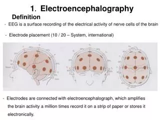
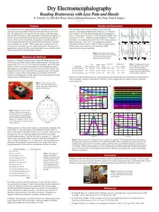
10. #1. 0. -10. 10. #2. 0. -10. 10. #3. 0. 200. -10. 10. #4. 0. -10. 10. 0. #5. 0. -10. 10. amplitude ( m V). #6. 0. -200. -10. 10. #8. 0. Fp. -10. -400. 10. Fp2. #9. Fp1. 0. -10. amplitude ( u V). #1. 10. -600. #10. 0. #2. -10. F7. F8. #3. 10.

E N D
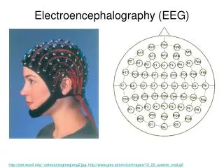
10 #1 0 -10 10 #2 0 -10 10 #3 0 200 -10 10 #4 0 -10 10 0 #5 0 -10 10 amplitude (mV) #6 0 -200 -10 10 #8 0 Fp -10 -400 10 Fp2 #9 Fp1 0 -10 amplitude (uV) #1 10 -600 #10 0 #2 -10 F7 F8 #3 10 #12 0 -800 F3 Fz F4 #4 -10 #5 10 #13 0 15 13 #6 12 14 -10 -1000 #8 0 2 4 6 8 10 12 #9 time (min) T4 10 C3 Cz C4 11 9 T3 8 #10 -1200 #12 7 2 40 0.08 #13 5 3 6 4 #1 #1 -1400 0 2 4 6 8 10 12 #2 #2 20 A2 Pz 0.07 time (min) #3 #3 P3 P4 T5 T6 #4 #4 0 #5 #5 0.06 1 #6 #6 -20 #8 #8 O1 #9 #9 0.05 O2 O -40 #10 #10 #12 #12 power spectral density (db/Hz) proportion of signal in 0.1 mV bins -60 0.04 #13 #13 -80 0.03 -100 0.02 -120 0.01 -140 -160 0 0 5 10 15 20 25 30 -3 -2 -1 0 1 2 3 frequency (Hz) amplitude (mV) Dry Electroencephalography Reading Brainwaves with Less Pain and Hassle E. Timothy Uy, Dik Kin Wong, Marcos Perreau Guimaraes, Wei Yang, Patrick Suppes Purpose Results and Discussion In conventional electroencephalography (EEG), scalp abrasion and use of electrolytic paste are needed to insure low-resistance between sensor and skin. By replacing this “wet” process with dry sensors, setup and cleanup time are drastically reduced. More importantly, the number and frequency of sessions are no longer limited by the amount of abrasion human scalp can tolerate. However, the unavailability of amplifiers with sufficiently low noise and high input impedance has held back the development of dry EEG sensors until the very recently1. While single-sensor comparisons of wet versus dry exist2, there has yet to be a multi-sensor study. Our goals are to quantitatively evaluate dry EEG sensors under multi-sensor conditions and to develop specifications for high fidelity recording. The classification rate for the best subject was 93 out of 100 sentences. The optimal bandpass-filter started at L = 1.25 Hz and had a width W = 21.25 Hz. Start and end points for calculating fit were s = 180 ms and e = 2200 ms. C4-T6 was the best channel. The search space (L, W, s, e, channel) was approximately 107. The next best subject, on a smaller grid, rated 27 out of 100. These results are highly significant, p value <10-10, and quantitatively similar to experiments using wet sensors3 (Table 2). Moreover, they suggest that dry sensors are as effective as wet electrodes in EEG experiments involving averaged data. Figure 3. Prototypes (gray) and test (dashed) waveforms for the best-fitting (top) and worst-fitting (bottom) sentences for the best subject. Materials and Methods Eight dry 1x Softsens™ sensors (Figure 1) from IBT (Redwood City, CA) were used to record EEG from five native English speakers. We placed the sensors at F8, T3, C3, Cz, C4, T4, T5 and T6 according to the 10-20 system (Figure 2). Prior to connection with Model 12 Grass Instruments (Quincy, MA) amplifiers, each output was low-pass filtered at 100 Hz. Signals were further filtered between 0.3 and 100 Hz and captured using a 16-bit analog-to-digital converter (ADC) card and Neuroscan (Sterling, VA) SCAN 4 software at a sampling rate of 1 kHz. Sensors were secured against the scalp using an elastic cap fabricated in our lab. Table 2. Comparison of wet and dry classification for best subject results. Mean and standard deviation for the null-hypothesis extreme statistic Y confirm that the results are highly significant. Inspection of single trial data, however, reveals artifacts such as spiking which were not present in conventional wet sensor recordings. Analysis of individual 5x Softsens™ sensors suggests that the artifacts were due to defective sensors (Figure 4). Figure 1. Close-up of dry sensor contact. The sensor makes contact with the scalp using a medical-grade stainless steel snap post. (a) (b) Anterior Figure 2. Bird’s-eye view of 10-20 system for EEG sensor placement. Locations in red, e.g., Cz, indicate dry sensor placement. Recorded bipolar pairs are indicated in blue by channel number, e.g., channel 1 = T5-T6. A wet sensor at A2 (green) was used as the dry sensor reference. (c) (d) Posterior Stimuli consisted of 100 true-false sentences concerning the geography of the world (Table 1). The 100 sentences were displayed in random order in a block. Each subject sat through 30 blocks over 12 sessions. Sentences were presented one word at a time using timing extracted from a previously recorded spoken sentence. After the last word of a sentence, a "?" appeared on the screen to prompt the subject to indicate whether the statement was "true" or "false" by pressing "1" or "2" respectively. The next sentence was presented 1500 ms after the offset of the last word. If the subject did not respond during the 1500 ms interval, an additional 1000 ms was added. Figure 4. Baseline noise of 11 5x Softsens™ sensors. (a) Data was captured at 1920 Hz immediately after battery insertion and digitally low-pass filtered at 30 Hz using a 10th order Butterworth IIR. Sensors are labeled by sensor ID. Sensors #1 and #5 appear stable. Sensors #4 and #12 are prone to spiking. (b) Signals from (a) were high-pass filtered at 0.3 Hz using a 6th order Butterworth IIR. All sensors except for #4 and #12 should be free from spiking and large amplitude fluctuations between 0.3 and 30 Hz. (c) Histograms generated from (b) show that underlying noise is Gaussian in nature. In addition, the spiking nature of #4 and #12 could not be determined from the histogram. (d) Power spectral density plots over the recording identify #4 and #12 as problematic. Table 1. Distribution of sentences by sentence template. X indicates a US or international city, and Y indicates a US state or a country. Each city, state or country appeared exactly twice in the 100 sentences, once on the left and once on the right. Conclusion Preliminary results show that dry sensors are feasible at least for experiments involving averaging. For use in single trial analysis, noise from each sensor should be analyzed over a time period proportional to experiment length. Sensors spiking over time, having wide histograms, or having unusual power spectral density should be rejected. Figure 5. Scalp abrasion in standard wet EEG. Having dry sensors means less pain and hassle for the researcher and the subject. For analysis, prototype and test waveforms for each of the 100 sentences were generated by averaging 15 trials for the prototype and the remaining 15 for the test. Each test waveform was compared to the set of prototypes, amongst which the best fitting prototype was selected. Fit was quantified using a minimum least squares measure. Classification rate is the rate at which the correct prototype is selected for a given test. Frequency and temporal windows were adjusted to maximize classification rate3. References • B. Alizadeh-Taheri, R. L. Smith, and R. T. Knight, "An active, microfabricated, scalp electrode array for EEG recording," Sensors and Actuators A, vol. 54, pp. 606-611, 1996. • A. Searle and L. Kirkup, "A direct comparison of wet, dry and insulating bioelectric recording electrodes," Physiological Measurement, vol. 21, no. 2, pp. 271-283, May 2000. • P. Suppes, B. Han, Z. Lu, “Brain-wave recognition of sentences,” PNAS¸ vol. 95, pp. 15861-15866, 1998. In addition, noise from dry 5x Softsens™ sensors was studied using a Cirrus-Logic (Austin, TX) CS5532 24-bit ADC. Data was sampled at 1920 Hz, imported into Matlab and low-pass filtered at 30 Hz.