Download
1 / 25
250 likes | 397 Vues
The Pluto System in the Context of Kuiper Belt Formation & Evolution. A. Morbidelli (OCA – Nice). THIS TALK WILL FOCUS ON THE DYNAMICAL ASPECTS OF THE KUIPER BELT EVOLUTION

E N D
The Pluto System in the Context of Kuiper Belt Formation& Evolution A. Morbidelli (OCA – Nice)
THIS TALK WILL FOCUS ON THE DYNAMICAL ASPECTS OF THE KUIPER BELT EVOLUTION IT WILL SET THE STAGE FOR BOTTKE’S TALK ON THE COLLISIONAL ASPECTS, WHICH HAVE MORE DIRECT IMPLICATIONS FOR THE PLUTO SYSTEM PUNCHLINE • Properties of the Kuiper belt that need to be explained in the framework of a dynamical evolution scenario • Misconception that said properties are explained by the radial migration of Neptune • Basic aspects of the giant planets dynamical evolution • The evolution of the Kuiper belt in the context of the giant planets evolution • A two-population model for the primordial proto-planetary disk
Orbital overview of the Kuiper belt Classical Resonant Scattered Detached
Coexistence of resonant and classical population; weird (a,e) distribution of the classical objects Trujillo et al. (2001): all resonances = ~10% of the classical population Kavelaars et al. (2009): 2/3 resonance = ~20% of the classical population
Coexistence of `hot’ and `cold’ classical populations, containing roughly the same number of D=100km objects (Brown, 2000)
PHYSICAL DIFFERENCES BETWEEN THE HOT AND COLD POPULATIONS OF THE CLASSICAL BELT: I) THE COLOR DISTRIBUTION Trujillo and Brown (2002), Tegler and Romanishin (2000), Doressoundiram et al. (2001)
PHYSICAL DIFFERENCES BETWEEN THE HOT AND COLD POPULATIONS OF THE CLASSICAL BELT: II) THE SIZE DISTRIBUTION Levison and Stern (2001) All of the biggest objects (Pluto, Quaoar, Ixion, Varuna, Chaos) are in the HOT population big small All bodies with H<5 have i>5o and have imed=19.7o
TNO magnitude (size) distribution Total mass estimate: ~0.01 M Bernstein et al. (2004)
THE MASS DEFICIT 30 Earth masses are expected to exist in the primordial 30-50 AU region because of: • Extrapolation of the surface density of solids incorporated in the giant planets • Necessity to grow the KBOs in a reasonable timescale • (Stern, 1996; Stern and Colwell, 1999; Kenyon and Luu 1998, 1999; Weidenshilling, 2003)
The misconception of Neptune’s migration Following Malhotra’s (1993, 1995) pioneering work on mean motion resonance capture, it is often believed that the properties of the Kuiper belt are explained by a smooth radial migration of Neptune. This model does not explain: the inclination distribution, the shape of the (a,e) distribution of the classical belt, the edge at the 1:2 MMR with Neptune, the mass deficit, correlations of colors and SFDs with inclination, the color distribution of plutinos…. BESIDES, THE PLANETS DID NOT MOVE IN A SMOOTH WAY….
When the giant planet where still embedded in a gas disk, Jupiter and Saturn should have been trapped in the 2/3 resonance and this prevented their migration to the Sun (Masset and Snellgrove, 2001; Morbidelli and Crida, 2007; Pierens and Nelson, 2008). Then, Uranus and Neptune should have been captured in resonances with Saturn and with themselves. Thus, the 4 planets should have reached reached a multi-resonant equilibrium configuration (Morbidelli et al., 2007). Resonance trapping is very common among extra-solar planet systems.
At the disappearance of the gas, under the influence of the planetesimal disk, the planets are eventually extracted from the resonances. But they are too close to each other to remain stable. So, rather than having a smooth planetesimal-driven migration, their radial displacement is abrupt, violent and involves a high-eccentricity phase
The instability phase might have occurred late, if the planetesimal disk was sufficiently far from the planets. This should have been the case if the LHB is related to this orbital instability event
We know that the radial displacement of the orbits of the planets was not a smooth migration process because: • It could not explain the eccentricities and inclinations of the planets • Even if the planets had crossed some resonance, only some secular modes could have been excited, not all of them (Morbidelli et al., 2009) • It would have taken ~10My and this long migration timescale would have left indelible scars in the asteroid belt, which are not observed (Minton and Malhotra, 2009; Morbidelli et al., 2010)
Thus, we need to investigate the evolution of the Kuiper belt in the context of the dynamical instability of the giant planets. • Two main aspects: • To reproduce the current orbital architecture of the giant planets in a dynamical instability scenario, the primordial trans-Neptunian planetesimal disk had to have 30-50 Earth masses and an outer edge at 30-35 AU (i.e. the current Kuiper belt was empty or at least it did not contain any population of significant mass) • The eccentricity of Netune at some point during his evolution was larger than 0.2 – 0.3
The Kuiper belt can be filled up to the 1:2 MMR, and an extended SD is formed, when Neptune is eccentric eNeptune=0.2, fixed
We did a series of new simulations where we forced the planets to behave as in the planet evolution simulations: Large e, damping, migration
We reproduce the (a,e) distribution fairly well simulation observation q=30AU q=30AU DLB95 stab. lim. DLB95 stab. lim.
We also reproduce the observed inclination distribution, although we have some deficit of large-i objects. KS test says distributions match at 50% confidence level model + biases observed
We see a correlation between initial location and final inclination that might explain the difference in physical properties of hot/cold pops.
SKETCH OF OUR ENVISIONED MODEL e,i SD Hot J Trojans Cold a ~34AU 40AU 50AU ~15AU
=0.4 (Jewitt et al., 2000; Szabo et al., 2007) The size distributions of the cold population and of the Trojans are the same! Real turn-over This implies that the apparent turnover of the size distribution of the cold belt is due to biases, and that the real turn-over should be at D~100km (in agreement with recent pencil beam surveys – Fuentes and Holman) Apparent turn-over due to biases But… why the Trojans don’t have the SFD of the Hot population?
Our interpretation of this (Morbidelli et al., 2009) Turnover H (~9) Real Hot population SFD Observable part of the hot population H of largest Trojan (~7.5) N N H H Inner disk Outer disk a
A quantitative model of the primordial trans-Neptunian disk (Morbidelli et al, 2009) q=-2; =0.4 TOTAL MASS = 35 Earth masses D q=-5.5 ; =1.1 q=-3 ; =0.6 H=9 H=6.5 Pluto size
conclusions • The evolution of the Pluto system should be seen in this context • Bill Bottke will elaborate on the collisional implications • Pluto, of course, should have formed in the inner part of the disk • Remember that the dynamical instability that led to the described events could have occurred late (if needed to explain the LHB) or early. In-situ constraints should help to decide on this.