Risk Analysis & Modelling
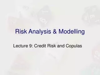
Risk Analysis & Modelling. Lecture 6: Value at Risk & Solvency II. www.angelfire.com/linux/riskanalysis RiskCourseHQ@Hotmail.com. Making Sense of Quantitative Risk. In an earlier lecture we looked at the Mean-Variance Model

Risk Analysis & Modelling
E N D
Presentation Transcript
Risk Analysis & Modelling Lecture 6: Value at Risk & Solvency II
www.angelfire.com/linux/riskanalysisRiskCourseHQ@Hotmail.com
Making Sense of Quantitative Risk • In an earlier lecture we looked at the Mean-Variance Model • We saw how we could calculate the Mean and Variance of the return on a portfolio from the statistical properties of the assets it contains • The Expected Return was relatively easy to interpret • The Variance or Standard Deviation was abstract and did not mean much other than to give a measure of the relative risk – the higher the variance the higher the risk
Value At Risk: Implying Potential Loss • People intuitively try to assess risk in terms of worst case scenarios • Information on how much you could lose on a portfolio over the next day, month or year makes much more sense to most people than an abstract statistic such a variance • Value at Risk originated in the RiskMetrics group at the investment bank JP Morgan in the early 1990s • It quantifies the worst case scenario in terms of the probability of observing outcomes worse than this scenario (ie the Quantile of the loss) • VaR is very closely related to the Probable Maximum Loss (PML) used to measure Underwriting Risks
Value At Risk Losses due to Random Movements in the Assets Value will only be greater than this some % of the time Random Asset Value Increases in Values (Profit) Decreases in Values (Loss) % Value at Risk
Measuring VaR From Historical Observations • Imagine we have some historical data (or simulated values) on the profits and losses experienced on an investment over a one year period • We believe that this historical data represents the future profits and losses we might experience • We could estimate the 5% VaR over the next year by locating the loss such that only 5% of the losses are worse (5% Empirical Quantile) • We could estimate the 1% VaR over the next year by locating the loss such that only 1% of the losses are worse (1% Empirical Quantile) • VaR is often calculated using statistical distributions…
VaR Assumption: Normally Distributed Returns • From an early lecture we discussed how we could use the Mean and Variance of the proportional change in the value of a portfolio (or asset) to assess the risk and return • If we assume these proportional changes or returns are Normally Distributed we can model the behaviour of a portfolios value by sampling random returns from a Normal Distribution with the appropriate mean and variance and applying the formula:
Since Value at Risk tries to measure the maximum loss we need to convert this into a model of the profit or loss • The random profit or loss (P) on holding an asset can be defined as: • The Value at Risk is simply the value for P that we will only observe outcomes (or losses) less than or equal to some percentage of the time • This value can be calculated by finding the appropriate Quantile for the Normally Distributed return r
Calculating VaR from the Return By finding the value that Returns will be less than or equal to 5% of the time we can calculate the value negative losses will be less than or equal to 5% of the time or the 5% VaR
Example VaR Calculation • The average return on the portfolio over the next year is 4% and the standard deviation is 7% • If we assume returns are normally distributed, we can use NORMINV to calculate the value such that the annual return will be less than or equal to 5% of the time (the 5% Quantile): =NORMINV(0.05,0.04,0.07) • This gives us a value of -0.07514 (-7.514%) • If the initial value of the portfolio was £10000 then the loss for this return would be -£751.4 (-0.07514 * 10000) over the next year • 5% of the time we will observe losses greater than £751.4 - this is the 5% VaR on the portfolio
5% VaR Calculation Diagram Only observe returns less than this 5% of the time CDF of returns with m = 0.04 and s = 0.07 0.05 -0.07514 5% VaR = -0.07514 * 10000 = -£751.4
VaR Review Question • The annual return on the portfolio is normally distributed with a mean of 6% and a standard deviation of 10% • The initial value of the portfolio is £250,000 • Calculate the 5% VaR over a 1 year horizon • Calculate the 1% VaR over a 1 year horizon
Normal vs Empirical CDF for Daily Returns on the FTSE Lower Tail Diverging
Locating Quantiles for the Normal Distribution • One useful feature of the normal distribution is its Quantiles can be located by simply taking a number of standard deviations from the mean • For example, the 5% Quantile for a normally distributed random variable is located 1.645 standard deviations below the mean • The 1% Quantile for a normally distributed random variable is located 2.326 standard deviations below the mean • The 0.5% Quantile of a normally distributed random variable is located 2.575 standard deviations below the mean • The number of standard deviations below the mean can be calculated using the CDF of a Standard Normal random Variable (Mean 0 and Standard Deviation of 1)
Location of Quantiles on the Normal Distributions PDF(X) s PDF(X) m -1.645*s s m -2.575*s m Lower 5% tail PDF(X) m Lower 0.5% tail s m -2.326*s m Lower 1% tail
5% Quantile for Normal Distribution with m = 0.04 and s = 0.07 The location of the 5% Quantile is 1.645 standard deviation below the mean 0.05 0.04 – 1.645 * 0.07 = -0.07515
VaR Formula • To calculate the 5% VaR over some time horizon we can simply apply VaR5%=V0.(m-1.645*s) • Where V0 is the initial value of the portfolio or asset, m is the mean of random return over the period and s is the standard deviation over the period • The 1% VaR formula is equal to: VaR1%=V0.(m-2.326*s)
Example VaR Formula Calculation • Let us apply these formula to our earlier example where the average return on the portfolio over the next year is 4% and the standard deviation is 7% over the year and the initial value of the portfolio is £10000 • Applying the 5% VaR fomula: VaR5%=10000*(0.04-1.645*0.07) VaR5%=10000*-0.07515 = -£751.5 • There is a slight difference because this is an approximation (1.645 should be 1.644853….) • This measures the maximum loss over one year because the mean and standard deviation of returns are measured over one year
Positive and Negative VaR • So far we have been calculating VaR as a negative value (signifying loss) • In practice it is often quoted as a positive number • This is achieved by multiplying the negative VaR measure by minus one • We can also adjust our formula to take this into account: VaR+X%=V0.(c*s-m) • Where c is the desired confidence interval (c = 1.645 for 5% VaR) • For the rest of the lecture we will use this VaR+ measure since this in the convention
Absolute vs Relative VaR Formula • So far our VaR calculation has measured the worst outcome by taking a number of standard deviations away from the mean, this is known as Absolute VaR: • This formula was based on the standard definition of profit and loss on an asset: • The formula for Relative Profit and Loss is relative to the expected return on the investment:
Using the relative measure, a profit is made when the future value is above its expected value, and a loss is made when it is below its expected value • Applying this definition we obtain: • Effectively this is equivalent to assuming that the average return mr is 0 • When to use Absolute or Relative VaR entirely depends on how you want to measure risk • Relative VaR produces a more conservative estimate of the worst loss since it does not allow any expected profit to offset losses • To calculate Relative VaR we only have to estimate the Variance of the return on the asset
VaR Review Question • The annual return on the portfolio is normally with a standard deviation of 15% • The initial value of the portfolio is £500,000 • Calculate the 5% Relative VaR over a 1 year horizon • Calculate the 1% Relative VaR over a 1 year horizon
Conditional Value at Risk (CVaR) • Another Measure of Value at Risk is CVaR or Conditional Value at Risk (also known as ETL or Expected Tail Loss) • It measures the average of all the losses beyond some Quantile for example the average of the worst 1% or 0.5% of losses • The loss provided by CVaR is always greater than the VaR measure at the same confidence level • CVaR has a number of advantages over traditional VaR
CVaR is the Averge in the Tail 5% CVaR is the Average of the Worst 5% of losses 5% VaR Loss Profit
Calculating CVaR for the Normal Distribution We can calculate CVaR for the Normal Distribution with by simply adjustment to the confidence interval c (c would be 1.64 for 5% VaR): Where PDFSN and CDFSN is the Probability Density Function and Cumulative Distribution Function for the Standard Normal (Normal with mean 0 and standard deviation of 1) We then apply this adjust confidence interval to standard VaR formula to obtain the equivalent CVaR:
For example, if we want to find the confidence interval for the 5% CVaR we can take the 5% VaR interval (1.64) and apply the adjustment: We could then see that the 5% Relative CVaR formula would be: REVIEW QUESTION: Calculate the CVaR 0.5% confidence interval based on the VaR 0.5% confidence interval of 2.575 then calculate the Relative CVaR 0.5% for a portfolio with an initial value of 10000 and a standard deviation of 0.07
Advantages of CVaR over VaR • Both VaR and PML (Probable Maximum Loss) are based on estimating the location of a single Quantile • Unlike CVaR and ETL they do not take into account what is taking place beyond that Quantile and this can lead to problems when used with Heavy Tailed distributions with Extreme Events in their tails • The first problem with VaR and PML is that in certain examples the loss measured can be very sensitive to small changes in the subjective confidence interval • CVaR and ETL are less sensitive because they are not just based on a single point • An example to highlight this issue is found on the “PML vs ETL” spreadsheet
Another problem is that for heavy tailed distributions the VaR on a portfolio of 2 assets (A and B) can be greater than the individual VaRs on the two assets, when this happens VaR violates Sub-Additivity: • This is an incoherent measure since in the most extreme case where the assets are perfectly positively correlated we expect the risk on the portfolio to simply be the sum of the individual risks: • CVaR (and ETL) are always Sub-Additive: • These problems do not occur on VaR calculations based on the Normal Distribution, and as we will see Solvency II is based on the Normal VaR model…
VaR and the Mean Variance Framework • One of the main uses of VaR is to estimate the risk on portfolios of assets • To calculate a portfolio’s Relative VaR we only have to calculate the variance of its return • In lecture 2 we saw that this can be calculated as:
We can also estimate the expected return on the portfolio and calculate the Absolute VaR: • Where C is the covariance matrix, w is the weight vector and E is the expected return vector
Breaking Down the Calculation c.V0 . * * * *
= * * * * * *
Alternative Value at Risk Calculation • The VaR on a portfolio can be Calculated by: • Where v is a vector of the Value at Risks for the individual assets and P is the correlation matrix between the assets • We note that the VaR on the portfolio of assets is less than the sum of the VaRs on the assets it contains due to diversification
Aggregating VaRs CORRELATION MATRIX (P) 1% VaR on Portfolio of A,B and C
What this Tells Us • What this equation is telling us is that we can derive the maximum loss on a portfolio of assets from maximum losses on the assets contained • The maximum total loss or VaR on the portfolio is less than the sum of the VaR’s on the individual assets because of the diversification effect • The extent of this diversification is determined by the correlation matrix
Review Question • You are working for a company that has two potential investments A and B. • The company estimates that the 0.5% VaR on investment A is £100,000 over the next year (based on a statistical model) and the 0.5% VaR on investment B is £70,000 over the next year (based a 1 in 200 worst case scenario) – the profitability of the two investments are believed to be independent or uncorrelated • The company says the maximum loss it is willing to take is £130,000 at a 0.5% confidence level, and since these two losses sum to £170,000 the company cannot invest in both • Why is just adding these losses incorrect and how would you calculate the 0.5% VaR across both investments?
Assumptions: Elliptical Distributions • We derived our risk Aggregation Formula using the Normal Distribution • But our Risk Aggregation Formula is not restricted to risks described by the Normal Distribution it will work for any Elliptical Distribution • Elliptical distributions are those for which the location of the Iso-Loss lines we drew earlier are Elliptical or spherical and this includes Students distribution which has heavy tails • Basically the trick works for elliptical distributions because that is what the correlation matrix and the quadratic form describes – ellipses and circles!
Visualising What is Happening VaR(A+B) = 130000 VaR A = 100000, VaR B = 83000, VaR(A+B) = 130000 When rA,B=0
SCR and Solvency II • Insurance Companies are required by Regulators to hold certainly levels of capital to protect policy holders • If the insurance company falls below these required levels costly regulatory intervention is enforced and ultimately the company can be declared Insolvent • In 2016 the European Union will be introducing a new Unified Risk Based Capital System called Solvency II • The Solvency Capital Requirement (SCR) in Solvency II requires Insurance Companies to hold sufficient capital such that they will only become insolvent 1 in every 200 years, or that over 1 year they are 99.5% likely to remain Solvent • From the perspective of the Balance Sheet this means that over a one year horizon the probability of Assets being worth less than Liabilities is only 0.5%
Capital Absorbs Adverse Shocks Adverse Shocks cause a decrease in Assets and increase in Liabilities which has been absorbed by the Insurers Capital Assets (A) Capital (C) Assets (A) Capital (C) Liabilities (L) Liabilities (L) The initial level of Capital or SCR is set such that it will absorb 99.5% of adverse movements in Assets and Liabilities
Calculating SCR from Scenarios • The Standard Model for Solvency II provides a number of worst case scenarios calibrated to a 1 in 200 year event called Shocks • For documentation of these Shocks see https://eiopa.europa.eu/consultations/qis/quantitative-impact-study-5/technical-specifications/index.html • For each Scenario or Shock the insurance company has to calculate how much capital it would need to absorb either a decrease in Assets or increase in Liabilities • If the insurer has an amount of capital equal to this loss then it would just be able to absorb this shock and remain solvent, this amount becomes the required level of capital or SCR
Market Risk Shock for Equities in Solvency II • An Insurance Company has £1 million invested in FTSE-100 stocks • In the QIS (Quantitative Impact Study) 5 the 1 in 200 or 99.5% worst case Scenario or Shock relating to this asset is that equities listed in EEA and OECD countries will drop by 30% • Under this scenario the company would have to have 30% of £1 million or £300,000 of Capital to absorb this loss, so the SCR for this risk is £300,000
SCR Assets drop by £300,000 Assets (A) SCR (£300000) Assets (A) Liabilities (L) Liabilities (L) Insurer just remains solvent after shock Under the Scenario or Shock the value of the assets will drop by £300,000 so the SCR required to absorb this is £300,000
Market Risk for Equities Shock 2 • The company also has £500,000 invested in emerging markets • Solvency II provides a separate 1 in 200 separate scenario for higher risk Hedge Funds and Equities in Emerging market investments that the value of the investment will drop by 40% • So in this scenario we would lose 40% of £500,000 or £200,000
Combining the Two Scenarios • We could simply add these two SCRs together to get the SCR required to absorb both these scenarios: £300,000 + £200,000 = £500,000 • As we saw adding scenarios in this way assumes they are perfectly correlated • The Solvency II system provides a correlation matrix set by the regulator that Insurance Company is expected to use to combine the SCRs
Equity Market Risk Correlation Matrix requity (Global) (Other) (Global) EEA and OECD Equities (Other) Emerging Markets, Hedge Funds
Solvency II Risk Aggregation Formula • The formula for the SCR on a portfolio of risks can be calculated as: • Where SCR is the aggregated Solvency Capital Requirement over the portfolio of risks, SCRV is a vector of the Solvency Capital Requirements on the individual risks and P is the correlation between these risks specified by the Regulatory Authority
SCR Aggregation SCRVequity= SQRT(MMULT(MMULT(TRANSPOSE(E5:E6),H5:I6),E5:E6)) = 469041