Heavy Traffic Limit Theorems for Real-Time Computer Systems
330 likes | 346 Vues
This presentation discusses heavy traffic limit theorems for real-time computer systems, focusing on workload modeling and analysis techniques. It covers the distinction between hard and soft real-time systems, goal formulation, and analysis methods such as heavy traffic analysis and lead-time profiling. The presentation also includes predictions for EDF deadline miss rates and discusses the use of various scheduling policies.

Heavy Traffic Limit Theorems for Real-Time Computer Systems
E N D
Presentation Transcript
Heavy Traffic Limit Theorems for Real-Time Computer Systems Presented by: John Lehoczky Carnegie Mellon Co-authors: B.Doytchinov, J.Hansen, L.Kruk, R. Rajkumar, C.Yeung, and H.Zhu Presented at WORMS04 April 19, 2004
Background: 1 • Real-time systems refer to computer and communication systems in which the applications/tasks/jobs/packets have explicit timing requirements (deadlines). • These arise in (e.g.): • voice and video transmission (e.g. video-conferencing) • control systems (e.g. automotive) • avionics systems
Background: 2 • We often distinguish different types of real-time systems or tasks: • Hard real-time: any failure to meet a deadline is regarded as a system failure. (e.g. avionics or control systems) • Soft real-time: deadline misses or packet loss is acceptable as long as it doesn’t reduce the QoS below requirements (e.g. multi-media applications).
For a given workload model we want: to predict the fraction of the workload that will miss its deadlines (end-to-end deadlines in the network case), to design workload scheduling and control policies that will ensure QoS guarantees (e.g. a suitably small fraction miss their deadlines), to investigate network design issues, e.g.: Number of priority bits needed Cost/benefit from flow tables Cost/benefit from keeping lead-time information Goals
Formulation • In the hard real-time formulation where no deadlines misses are permitted, one must adopt a worst case formulation: • task arrivals occur as soon as possible, • task services take on their maximum values, • task deadlines are as short as possible. • One must bound the worst case utilization. • But it average case utilization is substantially less than worst case utilization, the system will, on average, be highly underutilized.
Model • Multiple streams in a multi-node acyclic network. • Independent streams of jobs. • Jobs in a stream form a renewal process and have independent computational requirements at each node • For a given stream, each job has an i.i.d. deadline (different for different streams) • Node processing is EDF (Q-EDF), FIFO, PS, HOL-PS, Fixed Priority.
Analysis: 1 • In addition to tracking the workload at each node, we need to track the lead-time (= time until deadline elapses) for each task. • The dimensionality becomes unbounded, and exact analysis is impossible. • We resort to a heavy traffic analysis. This is appropriate for real-time problems. If we can analyze and control under heavy traffic, moderate traffic will be better.
Analysis: 2 • Heavy traffic analysis (traffic intensity on each node converges to 1) • One node – workload converges to Brownian motion. Multiple nodes, workload may converge to RBM (depending upon scheduling policy). • Conditional on the workload, lead-time profile converges to a deterministic form depending upon • flow deadline distributions, • scheduling policy • traffic intensity • Combining the lead-time profile with the equilibrium distribution of the workload process, we can determine the lateness fraction for each flow.
EDF Miss Rate Prediction EDF Deadline Miss Rate: =0.95 EDF scheduling Uniform(10,x) deadlines Internet Exponential : computed from the first two moments of task inter-arrival times and service times. : Mean Deadline Uniform
Motivation/Payoff CPU 1 CPU 2 Server 1 Server 1.1 Server 4 Stream 1 FIFO FIFO FIFO Server 2 Server 5 Stream 2 FIFO FIFO Server 3 Server 6 Stream 3 Stream 4 FIFO FIFO