Download
1 / 40
410 likes | 886 Vues
On the Pricing of Contingent Claims and the Modigliani-Miller Theorem. Chen Miaoxin. Introduction. Two assumptions. The theory of portfolio selection in continuous time has as its foundation two assumptions:

E N D
On the Pricing of Contingent Claims and the Modigliani-Miller Theorem Chen Miaoxin
Two assumptions • The theory of portfolio selection in continuous time has as its foundation two assumptions: • (a) the capital markets are assumed to be open at all times, and therefore economic agents have the opportunity to trade continuously; • (b) the stochastic processes generating the state variables can be described by diffusion processes with continuous sample paths (Chs 5 and 8). • If these assumptions are accepted, then the continuous-time model can be used to derive equilibrium security prices (Ch. 15).
Black and Scholes(1973) • B-S used the continuous-time analysis to derive a formula for pricing common-stock options. • The resulting formula expressed in terms of the price of the underlying stock does not require as inputs expected returns, expected cash flows, the price of risk, or the covariance of the returns with the market. In effect, all these variables are implicit in the stock’s price.
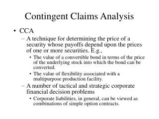
Contingent claim • The essential reason that the B-S pricing formula requires so little information as inputs is that the call option is a security whose value on a specified future date is uniquely determined by the price of another security (the stock). As such, a call option is an example of a contingent claim. • The same analysis could be applied to the pricing of corporate liabilities generally where such liabilities were viewed as claims whose values were contingent on the value of the firm. • Moreover, whenever a security’s return structure is such that it can be described as a contingent claim, the same technique is applicable.
Structure of this Ch. • In section 13.2, Merton derives a general formula for the price of a security whose value under specified conditions is a known function of the value of another security. • In section 13.3, the MM theorem that the value of the firm is invariant to its capital structure is extended to the case where there is a positive probability of bankruptcy. • In section 13.4, the author introduces the applications of contingent-claims analysis in corporate finance.
Assumptions 1-2 • 1 Frictionless markets There are no transactions costs or taxes. Trading takes place continuously in time. Borrowing and short-selling are allowed without restriction. The borrowing rate equals the lending rate. • 2 Riskless asset There is a riskless asset whose rate of return per unit time is known and constant over time. Denote this return rate by r.
Assumptions 3 • 3 Asset 1 There is a risky asset whose value at any point in time is denoted by V(t). The dynamics of the stochastic process generating V(·) over time are assumed to be describable by a diffusion process with a formal stochastic differential equation representation of
Assumptions 4 • 4 Asset 2 There is a second risky asset whose value at any date t is denoted by W(t) with the following properties: • For 0≤t<T, its owners will receive an instantaneous payout per unit time, • For any t (0≤t<T) • For t=T • Asset 2 is called a contingent claim, contingent on the value of Asset 1.
Assumptions 5-6 • 5 Investor preferences and expectations It is assumed that investors prefer more to less. It is assumed that investors agree upon σ2, but it is not assumed that they necessarily agree on α. • 6 Other There can be as many or as few other assets or securities as one likes.
Derivation • If it is assumed that the value of Asset 2 can be written as a twice continuously differentiable function of the price of Asset 1 and time, then the pricing formula for Asset 2 can be derived by the same procedure as that used in Merton (Section 12.2 and 12.3) to derive the value of risky debt.
Derivation • If W(t)=F[V(t),t] for 0≤t≤T and for then, to avoid arbitrage, F must satisfy the linear partial differential equation • To solve (13.1), boundary conditions must be specified. From Assumption 4, we have that • (13.1) together with (13.2a)-(13.2c) provide the general equation for pricing contingent claims.
The boundary conditions of B-S • While the function f, g, and h are required to solve for F, they are generally deducible from the terms of the specific contingent claim being priced. • For example, the original case examined by B-S is a common-stock call option with an exercise price of E dollars and an expiration date of T. If V is the value of the underlying stock, then the boundary conditions can be written as
Proposition • Suppose there exists a twice continuously differentiable solution to (13.1) and (13.2). Because the derivation of (13.1) used the assumption that the pricing function satisfies this condition, it is possible that some other solution exists which does not satisfy this differentiability condition. • The following alternative derivation is a direct proof that if a twice continuously differentiable solution to (13.1)and (13.2) exists, then to rule out arbitrage, it must be the pricing function.
Proof • Let F be the formal twice continuously differentiable solution to (13.1) with boundary conditions (13.2). • Consider the continuous-time portfolio strategy where the investor allocates the fraction w(t) of his portfolio to Asset 1 and 1-w(t) to the riskless asset. • Moreover, let the investor make net “withdrawals” per unit time (e.g. for consumption) of C(t).
Proof • If C(t) and w(t) are right-continuous functions and P(t) denotes the value of the investor’s portfolio, then the author has shown elsewhere (Equation 5.14) that the dynamics for the value of the portfolio, P, will satisfy the stochastic differential equation
Proof • Suppose we pick the particular portfolio strategy with • And the “consumption” strategy • Substituting from(13.5) and (13.6) into (13.4),we have that
Proof • Since F is twice continuously differentiable, we can use ITO lemma (Ch. 5) to express the stochastic process for F as • But F satisfies (13.1). Hence, we can rewrite (13.8) as • 注:
Proof • Let Q(t)≡F[V(t),t]. Then from (13.7)and (13.9), we have that • But (13.10) is a nonstochastic differential equation with solution • For any time t and where Q(0) )≡P(0)-F[V(0),0]. Suppose that the initial amount invested in the portfolio, P(0), is chosen equal to F[V(0),0].Then from (13.11) we have that
Proof • By construction, the value of Asset 2, W(t), will equal F at the boundaries V and , and at the termination date T. Hence, from (13.12), the constructed portfolio’s value P(t) will equal W(t) at the boundaries. Moreover, the interim “payments” or withdrawals available to the portfolio strategy, D2[V(t),t], are identical to the interim payments made to Asset 2. • Therefore, if W(t)>P(t) or W(t)<P(t), there will be an opportunity for intertemporal arbitrage. Hence, W(t) must equal F[V(t),t]
Advantages • Unlike the original derivation, this alternative derivation doesn’t assume that the dynamics of Asset 2 can be described by an ITO process, and therefore it does not assume that Asset 2 has a smooth pricing function. • Indeed, the portfolio strategy described by (13.5) and (13.6) involves only combinations of Asset 1 and the riskless asset, and therefore does not even require Asset 2 exists! The connection between the portfolio strategy and Asset 2 is that, if Asset 2 exists, then the price of Asset 2 must equal F[V(t),t] or there will be an opportunity for intertemporal arbitrage.
Introduction • In Section 12.5, Merton proved that, in the absence of bankruptcy costs and corporate taxes, the MM theorem obtains even in the presence of bankruptcy. • The method of derivation used in the previous section provides an immediate alternative proof.
Proof • Let there be a firm with two corporate liabilities: (a) a single homogeneous debt issue and (b) equity. The debt issue is promised a continuous coupon payment per unit time, C, which continues until either the maturity date of the bond, T, or the total assets of the firm reach zero. • The firm is prohibited by the debt indenture from issuing additional debt or paying dividends. At the maturity date, there is a promised principal payment of B to the debtholders. In the event that the payment is not made, the firm is defaulted to the debtholders, and the equity holders receive nothing. • So VL(t)=S(t)+D(t). In the event that the total assets of the firm reach zero, VL(t)=S(t)=D(t)=0. Also, by limited liability, D(t)/ VL(t)≤1
Proof • Consider a second firm with initial assets and an investment policy identical with those of the levered firm. However, the second firm is all-equity financed with total value equal to V(t). • Let the second firm have a dividend policy that pays dividends of C per unit time either until date T or until the value of its total assets reaches zero (i.e. V=0). • Let the dynamics of the firm’s value be as posited in Assumption 3 where D1(V,t)=C for V>0 and D1=0 for V=0
Proof • Let F(V,t) be the formal twice-continuously differentiable solution to (13.1) subject to the boundary conditions F(0,t)=0; F(V,t)/V≤1; and F[V(T),T]=min[V(T),B]. • Consider the dynamic portfolio strategy of investing in the all-equity firm and the riskless asset according to the “rules” (13.5) and (13.6) of Section 13.2 where C(t)=C. If the total initial amount invested in the portfolio, P(0), is equal to F[V(0),0], then from (13.12), P(t)=F[V(t),t].
Proof • Because both the levered firm and the all-equity firm have identical investment policies including scale, it follows that V(t)=0 if and only if VL(t)=0. And on the maturity date T, VL(T)=V(T). • By the indenture conditions on the levered firm’s debt, D(T)=min[VL(T),B]. But since V(T)= VL(T) and P(T)=F[V(T),T], it follows that P(T)=D(T). Moreover, since VL(T)=0 if and only if V(t)=0, it follows that P(t)=F(0,t)=D(t)=0 in that event. • Thus, by following the prescribed portfolio strategy, one would receive interim payments exactly equal to those on the debt of the levered firm. On a specified future date T, the value of the portfolio will equal the value of the debt. Hence, to avoid arbitrage or dominance, P(t)=D(t).
Proof • The proof for equity follows along similar lines. Therefore, p(t)=S(t). • If one were to combine both portfolio strategies, then the resulting interim payments would be C per unit time with a value at the maturity date of V(T). That is , both strategies together are the same as holding the equity of the unlevered firm. Hence, f[V(t),t]+F[V(t),t]=V(t). But it was shown that f[V(t),t]+F[V(t),t]=S(t)+D(t)≡VL(t). Therefore, VL(t)=V(t).
Comments • While the proof was presented in the traditional context of a firm with a single debt issue, the proof goes through in essentially the same fashion for multiple debt issues or for “hybrid securities” such as convertible bonds, preferred stock , or warrants.
MM theorem • The MM theorem holds that for a given investment policy the value of the firm is invariant to the choice of financing policy. It does not imply that the choice of financing policy will not influence investment policy and thereby affect the value of the firm. • Stiglitz(1972) and Merton (1973a): managers of firms with large quantities of debt outstanding may choose to undertake negative net-present-value projects that reduce the market value of the firm but increase the market value of its common stock. • Merton(1990b):discussion of the conflict between debtholders and equityholders over the investment and financing policies of the firm.
MM theorem • If the choice of securities issued by the firm can alter the tax liabilities of the firm, or if there are bankruptcy costs, then the MM theorem no longer obtains. But, as noted in Merton (1982a,1990a), the contingent-claims pricing technique can still be used to value corporate liabilities. • To do so, redefine V(t) as the pre-tax and pre-bankruptcy-cost value of the firm at time t and include as explicit liabilities of the firm both the government’s tax claim and the “deadweight” bankruptcy-cost claim. Because these additional “noninvestor” liabilities, like those held by investors, are entitled to specified payments that depend on the fortunes of the firm, the previous analyses of this section and Section 13.2 apply. Hence, for a fixed investment policy, the redefined “investor-plus-noninvestor” value of the firm will be invariant to the firm’s choice of financing policy.
MM theorem • Although the total investor-plus-noninvestor value of the firm does not depend on the financing choice, the allocation of that value between investor and noninvestor components does. Thus, for a given investment policy, the firm’s financing policy does “matter” to its management, debtholders, and stockholders.
Applications of Contingent-Claims Analysis in Corporate Finance
Advantages of CCA • (a) the relatively weak assumptions required for its valid application make CCA robust; • (b) the variables and parameters required as inputs in the valuation equation are either directly observable or reasonable to estimate; • (c) there are several computationally feasible numerical methods for solving the partial differential equations for prices; • (d) the generality of the methodology permits adaptation to a wide range of finance applications.
Applications of CCA • 1 The applications of CCA to the pricing of corporate liabilities: • Masulis(1976): analyze the effects on debt prices of changes in the firm’s investment policy. • Galai and Brennan and Schwartz(1976b) and Merton(1974): analyze the valuation of debt with call provisions. • Brennan and Schwartz(1977c,1980), Ingersoll(1977), and Merton (1970b):the pricing of convertible bonds. • Baldwin(1972) and Emanuel(1983b) evaluate preferred stock.
Applications of CCA • 2 The applications of CCA to the evaluation of loan guarantees and deposit insurance: • Gatto, Geske, Litzenberger, and Sosin(1980): study the pricing of mutual-fund insurance. • Kraus and Ross (1982): apply the continuous-time model to the problem of determining the fair rate of profit for a property-liability insurance company. • Bodie(1990): applies CCA to evaluate inflation insurance.
Applications of CCA • 3 The applications of CCA to the financial analysis of corporate employee-compensation plans, such as the evaluation of executive stock options and the evaluation of both explicit and implicit labor contracts that provide wage floors and employment guarantees, including tenure.
Applications of CCA • 4 The applications of CCA to capital-investment decisions and corporate strategy. • Traintis and Hodder(1990): CCA can be used to evaluate the benefits of a more broadly trained work force against the cost of the higher wages that must be paid whether this extra training is used or not. • Myers and Majd(1983): analyze the value of the option to abandon a project. • Myers(1977): CCA can be used to evaluate the option to choose when to initiate a project. Myers points out that recognition of this option is important to the proper evaluation of a firm’s growth opportunities.
Thanks to Wang Baohe