High Efficiency Video Coding
High Efficiency Video Coding. Kiana Calagari CMPT 880: Large-scale Multimedia Systems and Cloud Computing. Outline. Introduction Main concepts Improvements in coding efficiency Parallel processing Other features and details. Video Coding Standards. HEVC.

High Efficiency Video Coding
E N D
Presentation Transcript
High Efficiency Video Coding Kiana Calagari CMPT 880: Large-scale Multimedia Systems and Cloud Computing
Outline • Introduction • Main concepts • Improvements in coding efficiency • Parallel processing • Other features and details
HEVC • H.265orMPEG-H Part2: The new joint video coding standard • First edition finalized on Jan 2013 • Additional work planned to extend the standard … • 3D and multiview expected in 2014/2015 • Scalable extensions(SVC) expected in July 2014 • Range extensions (several color formats, increased bit depth)
HEVC • Mainly focus on: • Doubling the coding efficiency • Parallel processing architectures
HEVC 50% bit-rate reduction Same bandwidth, double the data ! Motivations: • Popularity of HD videos • Emergence of beyond HD format (4k x 2k , 8k x 4k) • High resolution 3D or multiview • More than 50% of the current network traffic is video HEVC is suitable for high resolution videos
HEVC Main Features and Improvements: • Coding Tree Structure • Intra Prediction • Motion Vector coding
Coding Tree Structure • Core of the coding layer: Coding Tree Units (CTU) instead of Macro Blocks (MB) Size of CTU can be larger that traditional MB
Coding Tree Structure • Coding tree blocks (CTBs): • Picture is partitioned into CTBs, each luma CTB covers a rectangular picture area of NxN samples (N=16, 32, 64) • Coding Tree Units (CTU): • The luma CTB and the two chroma CTBs, together with the associated syntax, form a CTU
Coding Tree Structure • Coding Blocks (CB): • CTB can be partitioned into multiple CBs • The syntax in CTU specifies the size and positions • Coding Units (CU): • The luma CB and the two chroma CBs, with the associated syntax, form a CU 8x8 ≤ CB size ≤ CTB size
Coding Tree Structure • The decision whether to code a picture area using inter or intra prediction is made at the CUlevel Quadtree Roots CTU CU TU PU
Coding Tree Structure • Prediction Blocks (PB): • Depending on the prediction type CBs can be spitted to PBs. • Each PB contains one motion vector (if in a P slice). • Prediction Unit (PU): • Again, the luma and chroma PBs, with the associated syntax, form a PU 4x4 ≤ PB size ≤ CB size
Coding Tree Structure • Transform Blocks (TB): • Blocks for applying DCT transform: 4x4 ≤ size ≤ 32x32 • Integer transform for 4x4 intra blocks. • Transform Unit (TU): • Again, the luma and chroma TBs, with the associated syntax, form a TU TB size ≤ CB size TB can span across multiple PBs
Coding Tree Structure • large CTB sizes are even more important for coding efficiency when higher resolution video are used • large CTB sizes increase coding efficiency while also reducing decoding time.
Intra Prediction • What is Intra Prediction?
Intra Prediction • Prior to HEVC
Intra Prediction • HEVC supports : • 33 directional modes • planar (surface fitting) • DC prediction (flat) • Using 4N+1 spatial neighbours • Extrapolating samples for a given direction
Motion Vector coding • There are two methods for MV prediction: • Merge Mode • Advanced Motion Vector Prediction (AMVP) (instead of sending the whole motion vector each time)
Motion Vector coding Merge Mode • A candidate list of motion parameters is made for the corresponding PU (Using spatial and temporal neighbouring PBs) • No motion parameters are coded, only the index information for selecting one of the candidates is transmitted • Allows a very efficient coding for large consistently displaced picture areas. (Combined with large block sizes)
Motion Vector coding Advanced Motion Vector Prediction (AMVP) • AMVP is used when an inter coded CB is not coded using the merge mode • The difference between the chosen predictor and the actual motion vector is transmitted… • … along with the index of the chosen candidate
Parallel Processing Tools Motivation: • High resolution videos • HEVC is far more complex than its prior standards • Since we have parallel processing architectures, why not use it !
Parallel Processing Tools • Slices • Tiles • Wavefront parallel processing (WPP) • Dependent Slices
Slice • Slices are a sequence of CTUs that are processed in the order of a raster scan. Slices are self-contained and independent. • Each slice is encapsulated in a separate packet.
Tile • Self-contained and independently decodable rectangular regions. • Tiles provide parallelism at a coarse level of granularity. Tiles more than the cores Not efficient Breaks dependencies
Wavefront Parallel Processing • A slice is divided into rows of CTUs. Parallel processing of rows. • The decoding of each row can be begun as soon a few decisions have been made in the preceding row for the adaptation of the entropy coder. • Better compression than tiles. Parallel processing at a fine level of granularity. No WPP with tiles !!
Dependent Slices • Separate NAL units but dependent (Can only be decoded after part of the previous slice) • Dependent slices are mainly useful for ultra low delay applications Remote Surgery • Error resiliency gets worst • Low delay • Good Efficiency Goes well with WPP
Comparison • Slice vs Tile • Tile vs WPP
Slice vs Tile • Tiles are kind of zero overhead slices • Slice header is sent at every slice but tile information once for a sequence • Slices have packet headers too Each tile can contain a number of slices and vice versa • Slices are for : • Controlling packet sizes • Error resiliency • Tiles are for: • Controlling parallelism (multiple core architecture) • Defining ROI regions
Tile vs WPP • WPP: • Better compression than tiles • Parallel processing at a fine level of granularity But … • Needs frequent communication between processing units • If high number of cores Can’t get full utilization • Good for when: • Relatively small number of nodes • Good inter core communication • No need to match to MTU size • Big enough shared cache
Other Features and Details • In-loop filters New SAO • Special coding modes • Profiles and Levels • Merge mode and Non-merge mode • Intra Prediction • Inter Prediction
In-loop Filters • Deblocking Filter (DBF) • SAO
In-loop Filters • Deblocking Filter • Reduces the blocking artifacts (due to block based coding) • Only applied to samples adjacent to PU and TU boundaries and aligned with the 8x8 sample grid • Controlled by the SPS and slice headers
In-loop Filters • Deblocking Filter • 3 Strengths : • Strength 2: If one of the blocks is intra coded • Strength 1: If any of the below • Strength 0: DBF not applied • At least one transform coefficient is non-zero • The references of the two blocks are not equal • The motion vectors are not equal
In-loop Filters • Deblocking Filter • According to the strength and average quantization parameter: • 2 cases for chroma: Normal filtering (if Strength >1) or No filtering • 3 cases for luma: • No filter • Weak filter • Strong filter
In-loop Filters • Deblocking Filter • Processing order: The filtering process can be done in parallel threads • 1st ) Horizontal filtering For vertical edges • 2nd ) Vertical filtering For horizontal edges
In-loop Filters • SAO • New in HEVC • After the deblocking filter • Applies to all samples satisfying the conditions • Performed on a region basis
In-loop Filters • SAO • Modifies Samples by adding an offset • The offset is based on look-up table values • Per CTB Type_ID=0 No SAO Type_ID=1 Band offset Type_ID=2 Edge offset
In-loop Filters • SAO • Band offset: Depends on Offset valueSample amplitude Full sample range Uniformly split into 32 bands 4 consecutive bands Have a + or – band offset
In-loop Filters • SAO • Edge offset: • 4 types • 5 categories (for classifying each sample)
In-loop Filters • SAO • Edge offset: Based on the category A value from the look-up table Categories 1, 2 : Negative offset Categories 3, 4 : Positive offset
Special Coding Modes • 3 special modes: • I_PCM • Lossless mode • Transform skipping mode
Special Coding Modes • I_PCM: samples are directly represented Prediction Transform Quantization Entropy For noise-like signals Extremely unusual signal characteristics Bypassed
Special Coding Modes • Lossless mode: residuals are directly fed to entropy Transform Quantization In-Loop filters Bypassed
Special Coding Modes • Transform skipping: Transform Improves compression for some videos such as computer generated images Bypassed
Profiles and Levels • Profile : A set of coding tools and algorithms that can be used • Level: Puts constraints on certain key parameters
Profiles and Levels • 13 levels • 8 of them have 2 tiers Main tier High tier Higher max bit rate For more demanding app.s
Profiles and Levels • 3 Profiles • Main: all-purpose 8 bit per pixel • Main 10: 10 bit per pixel where very high quality is critical • Main still picture: subset of main just a single still picture
Merge Mode • Candidates ? Spatial Availability check: {a1 , b1 , b0 , a0 , b2}