Download
1 / 77
770 likes | 785 Vues
Explore the study of MHD turbulence in the solar wind at the Advanced School in Space Environment 2006. Learn about the self-similarity and power laws observed in interplanetary fluctuations, as well as the impact of Alfvénic turbulence on solar wind heating and particle acceleration.

E N D
Advanced School in Space Environment - ASSE 2006: SOLAR-TERRESTRIAL PHYSICS 10-15 September 2006, L’Aquila, Italy Observing MHD Turbulence in the Solar Wind by R. Bruno INAF-IFSI, Rome, Italy
Study by Leonardo da Vinci (1452-1519) Related to the problem of reducing the rapids in the river Arno in Florence “Turbulence still remains the last major unsolved problem in classical physics.”Feynman et al. (1977) “Turbulence is like pornography. It is hard to define, but if you see it, you recognize it immediately.” G.K. Vallis (1999)
TURBULENCE Space and time chaotic behavior of a fluid flow The legacy of A.N. Kolmogorov (1903-1987)
The first feature we notice in interplanetary fluctuations is an approximate self-similarity when we look at different scales Scales of days Scales of hours and minutes Scales of seconds
self-similarity implies power-laws The field v(l) is invariant for a scale transformation lrlif there exists a parameter m(r) such that: The solution of this relation is a power law: v(l)=Clhwhere h=-logrm(r)
As a matter of fact, interplanetary fluctuations do show power laws Scales of fractions of AUs f-5/3 fc A typical IMF power spectrum in interplanetary space at 1 AU [Low frequency from Bruno et al., 1985, high freq. tail from Leamon et al, 1999]
Spectral index of turbulent phenomena is universal Scales of fractions of AUs Scales of cms f-5/3 fc A typical IMF power spectrum in interplanetary space at 1 AU [Low frequency from Bruno et al., 1985, high freq. tail from Leamon et al, 1999] Laboratory experiment on turbulence with low temperature helium gas flow [Maurer et al., 1994]
The phenomenology at the basis of these observations follows the energy cascade á la Richardson in the hypothesis of homogeneous and isotropic turbulence = energy transfer rate integral scales inertial range ~k-1 dissipation scales homogeneous=statistically invariant under space translation isotropic=statistically invariant under simultaneous rotation of dvand
K41theory and k-5/3 scaling (A.N. Kolmogorov,1941) 1 1 v1 4 3 3 4 eddy turnover time (generation of new scales) v2 2 2 if edoesn’t depend on the scale
Turbulence is the result of nonlinear dynamics and is described by the NS eq. Incompressible Navier-Stokes equation u velocity field P pressure n kinematic viscosity nonlinear dissipative For large Renon-linear regime
Turbulence is the result of nonlinear dynamics and is described by the NS eq. Incompressible Navier-Stokes equation u velocity field P pressure n kinematic viscosity nonlinear nonlinear dissipative dissipative Hydromagnetic flows: same “structure” of NS equations Elsässer variables z+ z- <B>
Turbulence is the result of nonlinear dynamics and is described by the NS eq. Incompressible Navier-Stokes equation u velocity field P pressure n kinematic viscosity nonlinear nonlinear dissipative dissipative Hydromagnetic flows: same “structure” of NS equations Nonlinear interactions and the consequent energy cascade need both Z+ and Z-
Definition of the Elsässer variables outward propagating wave B0 k B0 inward propagating wave k
Definition of the Elsässer variables outward propagating wave B0 k B0 inward propagating wave k
Different origin for Z+ and Z- modes Alfvénic radius VSW = VA VSW < VA solar wind solar wind VSW > VA 15~20 Rs VSW > VA Only Outwardwaves escape the region inside the Alfvénic radius. Outside the Alfvénic radius both waves are carried away by the solar wind. interplanetary space outward waves: solar origin + local origin inward waves: local origin only
Alfvénic correlations in the solar wind fast solar wind slow solar wind
Alfvénic correlations in the solar wind • The solar wind is the most accessible medium in which to study collisionless MHD turbulence. • The solar wind turbulence, within fast wind, has a strong Alfvénic character (Alfvénic modes have a longer lifetime than other MHD modes). • Alfvénic turbulence • contributes to solar wind heating and acceleration • accelerates particles to high energies • affects cosmic ray propagation In the following we will concentrate on Alfvénic turbulence
When an MHD fluid is turbulent, it is impossible to know the detailed behaviour of v(x,t) and b(x,t), the only description available is the statistical one. Very useful is the knowledge of the invariants of the ideal equations of motion (dissipative terms ~ 0 ) There are three quadratic invariants of the ideal system (Frisch et al., 1975) Total energy Magnetic helicity Cross-helicity
where b is in Alfvén units 1) the total energy per unit density E 2) the cross helicity Hc where B is defined via 3) the magnetic helicity Hm The integrals of these quantities over the entire plasma containing regions are the invariants of the ideal MHD equations
However, it is more convenient to use the normalized expressions for cross-helicity and magnetic helicity σc and σm can vary between +1 and -1 The sign of σc indicates correlation or anticorrelation between δv and δb The sign of σm indicates left or right hand polarization
Definitions and invariants using Elsässer variables fields Second order moments e+ and e- energy Kinetic energy Magnetic energy Cross-helicity
Elsässer ratio Alfvén ratio Normalized parameters Normalized cross-helicity Normalized residual energy
for an Alfvén wave: rA=eV/eB=1 C=(e+-e-)/(e++e-) =1 R=(eV-eB)/(eV+eB)=0
Helios • Two spacecraft, launch 1974 & 1975 • ecliptic orbit • perihelion : 0.29AU • aphelion: 1.0 AU • Provide measurements of solar wind at an early stage
Interplanetary data Eclipse 29.03.06, courtesy of G. Fardelli
MHD turbulence: wind speed dependence and radial(time) evolution on the ecliptic
Solar wind turbulence: experimental evidence of non-linear cascade Non-linear interactions still active between 0.3 and 1 AU first k-5/3 spectrum Coleman, Ap. J., 153, 371, 1968 Helios 2 data
e+ and e– spectra vs. wind speed • Outward fluctuations (e+) are dominant within fast wind. • e+~ e- within slow wind • Notice the value of the spectral slope towards a f –5/3 regime in slow wind. • (Helios data) Marsch and Tu, JGR, 95, 8211, 1990
e+ and e– spectra vs. radial distance for fast wind Fast wind 0.3 AU 0.9 AU For increasing distance the e+ and e– spectra approach each other (e+ decreases faster than e– ) At the same time the spectral slopes evolve, with the development of an extended f –5/3 regime. (Helios data) e+ e+ f –1 f –5/3 e– e– Marsch and Tu, JGR, 95, 8211, 1990
e+ and e– spectra vs. radial distance for slow wind Slow wind 0.9 AU 0.3 AU e+ e+ No much radial evolution spectral slopes always close to f –5/3 (Helios data) e- e- f –5/3 f –5/3
Elsässer ratio vs. radial distance rE = e–/e+ Fast wind 0.3 AU 0.9 AU The Elsässer ratio increases going from 0.3 to 0.9 AU. However, its value depends on the frequency range (Helios data) Marsch and Tu, JGR, 95, 8211, 1990
Elsässer ratio at large distance rE = e–/e+ Fast wind From hourly variances of z+ andz- Further ecliptic observations do not indicate any clear radial trend for the Elsässer ratio between 1 and 5 AU. (Ulysses data ecliptic phase) Bavassano et al., JGR, 106, 10659, 2001
Alfvén ratio vs. radial distance rA = ev/ eb Fast wind 0.9 AU 0.3 AU Bruno et al., JGR, 90, 4373, 1985, Marsch and Tu, JGR, 95, 8211, 1990 (Helios data) Going from 0.3 to 0.9 AU the Alfvén ratio, at hourly frequencies, decreases from ~1 to ~0.5.
Alfvén ratio at large distances rA = ev/ eb Fast wind radial variation of the Alfvén ratio rA as observed by Helios and Voyagers between 0.3 and 20 AU. At MHD scales (red line), after the fast decrease inside 1 AU, rAremains nearly unchanged; rA~0.5. (Helios and Voyagers data) Roberts et al., JGR, 95, 4203, 1990
First conclusion MHD turbulence in fast wind evolves with distance towards fully developed turbulence MHD turbulence in slow wind does not suffer radial evolution (already fully developed at 0.3 AU)
Which mechanism does generate turbulence in the ecliptic?
The 6 lowest Fourier modes of B and V define the shear profile Turbulence generation on the ecliptic: velocity shear mechanism(Coleman1968) The z+ spectrum evolves slowly Alfvén modes added • Solar wind turbulence may be locally generated by non-linear MHD processes at velocity-shear layers. • Magnetic field reversals speed up the spectral evolution. T=3 ~ 1 AU This process might have a relevant role in driving turbulence evolution in low-latitude solar wind, where a fast-slow stream structure and reversals of magnetic polarity are common features. Az– spectrum is quickly developed at high k 2D Incompressible simulations by Roberts et al., Phys. Rev. Lett., 67, 3741, 1991
A new laboratory: the polar wind Ulysses, the first spacecraft able to explore the heliosphere at high latitudes (up to 80°), has allowed us to study Alfvénic turbulence under a different solar wind regime, the polar wind. McComas et al., GRL, 25, 1, 1998
Ulysses • Launched in 1990 and still operating • perihelion : 1.3AU • aphelion: 5.4 AU • Latitudinal excursion: 82°
Polar wind features The presence of a polar wind depends on solar activity. At LOW activity the polar wind fills a large fraction of the heliosphere. In contrast, polar wind almost disappears at HIGH activity. L O W HIGH McComas et al., GRL, 29 (9), 2002 The polar wind,a relatively homogeneous environment,offers the opportunity of studying how the Alfvénic turbulence evolves under almost undisturbed conditions.
Polar wind: spectral evolution The development of a turbulent cascade with increasing distance moves the breakpoint between the f–1 and f –5/3 regimes to larger scales. Power spectra of z+ and z– at 2 and 4 AU in polar windclearly indicate a spectral evolution qualitatively similar to that observed in ecliptic wind. f –1 z+ polar wind 4 AU polar wind 2 AU z– f –5/3 Goldstein et al., GRL, 22, 3393, 1995
Spectral breakpoint: a comparison with ecliptic wind polar wind In the polar wind the breakpoint is at smaller scale than at similar distances in the ecliptic wind. Thus, spectral evolution in the polar wind is slower than in the ecliptic wind. (data from: Helios, IMP, Pioneer, Voyager, Ulysses) Horbury et al., Astron. Astrophys., 316, 333, 1996
Polar wind: Elsässer and Alfvén ratios vs. radial distance After an initial increase, rEbecomes almost constant (around 0.5). The predominance of outward modes (z+) is preserved as far as 5 AU. The imbalance in favour of the magnetic energy does not go beyond a value of ~0.25 for rA. rE = e–/e+ rA = ev/ eb (data from Ulysses)
Radial dependence of e+ and e– Ulysses polar wind observations show that e+ exhibits the same radial gradient over all the investigated range of distances. In contrast, e– shows a change of slope at ~2.5 AU. Notice the good agreement of the Ulysses gradients with Helios observations in the trailing edge of ecliptic fast streams. Ulysses Helios (data from Helios and Ulysses) Bavassano et al., JGR, 105, 15959, 2000
Turbulence generation in the polar wind: parametric decay • In the polar wind there aren’t strong velocity gradients velocity shear mechanism is not relevant. • parametric decay seems to work much better. A large amplitude Alfvén wave decays into three daughter waves, two Alfvénic ones (forward and backward propagating) and one compressive. Energy mainly goes to the backward Alfvénic mode and to the compressive mode.
Turbulence generation in the polar wind: parametric decay • Numerical Simulations of the non-linear growth of parametric decay (e.g., see Malara et al., Phys. Plasmas, 7, 2866, 2000and Del Zanna, Geophys. Res. Lett., 28, 2585, 2001) have shown that the final state strongly depends on the value of (thermal to magnetic pressure ratio). • For <1 the instability completely destroys the initial Alfvénic correlation. • For =1 (a value close to solar wind conditions) the instability is not able to go beyond some limit in the disruption of the initial correlation between velocity and magnetic field fluctuations. Final state is C~0.5
Malara et al., Phys. Plasmas, 7, 2866, 2000 The parametric instability for =1 The decay ends in a state in which the initial Alfvénic correlation is partially preserved. The predicted cross-helicity behaviour qualitatively agrees with that observed by Ulysses. Ulysses