Download
1 / 38
390 likes | 553 Vues
Computing Fundamentals 1 Lecture 1. Lecturer: Patrick Browne http://www.comp.dit.ie/pbrowne/ Room K308 Based on Chapter 1. A Logical approach to Discrete Math By David Gries and Fred B. Schneider. Equational logic. State is a list of variables with associated values.

E N D
Computing Fundamentals 1Lecture 1 Lecturer: Patrick Browne http://www.comp.dit.ie/pbrowne/ Room K308 Based on Chapter 1. A Logical approach to Discrete Math By David Gries and Fred B. Schneider
Equational logic • State is a list of variables with associated values. • Evaluation of an expression E in a state is performed by replacing all variables in E by their values in the state and then computing the value of the resulting expression. For example: • Expression x – y + 2 • State (x,5),(y,6) • Gives 5 – 6 + 2 • Evaluates to 1 • An expression may consists of constants, variable, operations and brackets.
Equational logic • Theories in mathematical logic are defined by their axioms and inference rules (e.g. equational logic). • An axiom isa distinguishedexpression that cannot be proved or disproved. • An inference rule is avalid argument which permits the substitution of expressions in the steps of a formal proof. • A theorem is either an axiom or an expression, that using the inference rules, is proved equal to an axiom or a previously proved theorem.
Textual Substitution • Let E and R be expressions and let x be a variable then • E[x := R] • Denotes an expression that is the same as E but with all occurrences of variable x replaced by R. • Textual substitution only replaces variables not expressions, but the variables can be replaced by expressions. The symbol ‘:=‘ indicates substitution (LHS replaced by RHS). • Textual substitution has a higher precedence than any other operator.
Inference Rule The inference rule provides a mechanism for deriving "truths" or theorems. A theorem is an expression that is true in all states. The inference rule is written as follows: (Expression or list of Expressions) Epremise/hypothesis if true Rconclusion then also true
Inference Rule Substitution • Textual substitution can be considered as inference rule, which provides a syntactic mechanism for deriving ‘truths’, or theorems. Theorems correspond to expressions that are true in all states. An inference rule consists of a list of expressions, called its premises or hypotheses, above a line and an expression, called its conclusion, below the line. It asserts that if the premises are theorems, then the conclusion is a theorem. The inference rule called substitution uses an expression E , a list of variables v , and a corresponding list of expressions F (next slide).
Inference Rule Substitution • Inference Rule Substitution (IRS) uses an expression E, a list of variables v and a corresponding list of expressions F: • (1.1) Substitution: • This rule asserts that if expression E holds in all states then so does E with all occurrences of the variablev replaced with corresponding expression F. The symbol ‘:=‘ indicates substitution (LHS replaced by RHS)..
Inference Rule Substitution(1.1) Epremise/hypothesis if true E[v := F]conclusion then also true expression E , a list of variables v, and a corresponding list of expressions F This rule asserts that if expression E is a theorem, then so is E with all occurrences of the variables of v replaced by the corresponding expressions of F.
Inference Rule Substitution(1) • If we know x + y = y + x in all states, then IRS allows us to conclude that b + 3 = 3 + b. • After substitution
Inference Rule Substitution(1) E is 2•x/2 = x Use inference rule substitution to form the inference rule 2•x/2 = x (2•x/2 = x)[x := j+5] after substitution 2•x/2 = x 2•(j+5)/2 = j+5
Equality • At the syntactic (or symbol level) the RHS and LHS of 2•x/2=x are not equal. However, their values are equal. • One way equality can be characterised in terms of expression evaluation: • Evaluation of the expression X = Y in a state yields the value true if expressions X and Y have the same value and yields false if they have different values. • Definition: iff is used as an abbreviation for “If and only if”; b iff c holds provided (i) b holds if c holds and (ii) c holds if b holds.
Equality • Another way of looking at equality is to use laws that allow us to show expressions are equal without evaluating them. • A collection of such laws can be regarded as a definition of equality, provided that two expressions have the same value in all states if and only if (iff) one expression can be translated into the other according to these laws.
Four laws for Equality • Reflexivity: x = x • Symmetry: (x=y) = (y=x) • Transitivity: • Leibniz: Leibniz says: Two expressions are equal in all states iff replacing one by the other in any expression E does not change the value of E (in any state).
Leibniz • Two expressions are equal in all states iff replacing one by the other in any expression E does not change the value of E (in any state).
Leibniz • The variable z is used in the conclusion because textual substitution is defined for the replacement of a variable but not for the replacement of an expression. In one copy of E, z is replace by X, and in the other copy it is replace by Y. Effectively, this use of the variable z allows replacement of an instance of X in E[z:= X] by Y, while still preserving the same value of E
Leibniz (See lab 2) • Assume b+3 = c+5 holds in all states. • We can conclude that adding d to both sides d+b+3=d+c+5 holds by: X: b+3 Y: c+5 E: d+z z : z After substitution
Semantics of variables, equality & Identity Variables in Python & CafeOBJ >>> x = 99999 >>> y = 99999 >>> x == y True >>> x is y False >>> x = y >>> x is y True Equal X:Nat Identical (Python is) x = y x y 99999 99999 0, 1, 2 , 3 , …. 99999 Variables in some programming language Some points: CafeOBJ variables do not match the above (left) conventional view of variables. In CafeOBJ a variable is constrained to range over a particular sort or kind (a domain). A variable is not considered equal to a particular element in the domain. In contrast to programming languages real world objects are unique, so we may need different concepts of equality and identity for real world objects than computational objects.
Functions • Function application can be defined in terms of textual substitution. Let g.z: E (expression e.g. z + 1) define a function g, then function application g.X is defined by: g.X = E[z := X] Python >>> def g(z): return z + 1 >>> g (3) 4
Fibonacci Function in Python and CafeOBJ Function Name Formal parameter CafeOBJ mod* FIB { pr(NAT) op fib : Nat -> Nat var N : Nat eq fib(0) = 0 . eq fib(1) = 1 . ceq fib(N) = fib(p(N)) + fib(p(p(N))) if N > 1 .} Start CafeOBJ @ cmd. prompt in fib.cafe open FIB . red fib(14) . def fib(n): if n == 0: return 0 elif n == 1: return 1 else: return fib(n-1) + fib(n-2) fib(14) Actual argument
Python function definition def g(z) : return (z + 1) Function application g(6) Functions • Function application can be defined in terms of textual substitution. Let g.z: Expression • Define a function g, then function application g.X is defined in general by: g.X = E[z := X] In this case: g.6 = E[z := 6] (6 is substituted for z)
Functions • This close correspondence between function application and textual substitution suggests that Liebniz links equality and function application:
In computing and mathematics there is a lot of notation! Notation 3 Notation 2 Notation 1 Notation 4
Reasoning with Leibniz’s rule • Leibniz allows the substitution of equals for equals in an expression without changing the value of that expression. We can demonstrate that two expressions are equal as follows: E[z:=X] = <X=Y> E[z:=Y] Explanation of proof step Expressions Variables
2 Notations for Leibniz’s rule • Leibniz says: Two expressions are equal in all states iff replacing one by the other in any expression E does not change the value of E (in any state). Premise E[z:=X] <X=Y> = <X=Y> E[z:=X]=E[z:=Y] E[z:=Y] Conclusion • The first and third lines on the left are the equal expressions of the conclusion in Leibniz. • In notation on left the middle line is the premise.
Reasoning with Leibniz’s rule • Recall John and Mary’s apples: [eq1] m = 2 * j and [eq2] m/2 = 2 * (j – 1) • Using Leibniz: [eq2] m/2 = 2 * (j – 1) = <using [eq1] m = 2 * j equation in terms of j> [eq3] (2*j)/2 = 2 * (j – 1) • From arithmetic, the following holds in every state: 2*x/2 = x • Continuing from above: 2*j/2 = 2 * (j – 1) = < 2*j/2 = j , can put j on LHS> j = 2*(j – 1)
Reasoning with Leibniz’s rule • Solve the following for j: j = 2*(j – 1) • giving: j = 2j – 2 j = 2 • We can reduce equations to value (or answer), or at least to their simplest possible form (SPF). • An example of SPF J = Y * (J – 1) J = Y * J – Y * 1 J = Y * J - Y • Without additional information we can go no further.
The assignment statement • In a procedural programming language the execution assignment statement looks like: (1.10) x := E (x becomes E) • Where x is a variable and E is an expression. This does not say that x is mathematically equal to E. Also, it is not a test for equality. The assignment statement in some programming languages is the same symbol as used for textual substitution (i.e. :=)
The assignment statement • A Hoare Triple is of the form {P}S{Q} where P is a precondition, Q is a post-condition and S is a statement. • Example of a procedural language + pre/post condition • {x=0} x := x+1 {x > 0} • is VALID iff execution of x:=x+1 in any state where x=0 results in a state where x>0. • This provides a logical scaffolding or logical framework for procedural programs (e.g. written in C). The framework is added to the program, the program does not include the logical framework.
The assignment statement in a procedural programming language. • (1.12) Definition of Program Assignment • {R[x:= E]} x:= E {R}. • This allows us to compute the pre-condition from the post-condition and assignment. • Suppose we want to use the assignment x:=x+1 and we want a post condition of x>4. Then R is x>4 so the pre-condition is (x>4)[x:=x+1] which after substitution gives x+1>4 or x>3. This is substitution This is assignment This is substitution
The assignment statement in a procedural programming language. Working through the last example in detail: {R[x:=E]} x:=E {R} {?} x:=x+1 {x>4} • R is x>4, • Assignment/substitution is x:=x+1 • pre-condition is {R[x:=E]} x>4[x:= x+1] substitution gives x+1 > 4 or x > 3.
Substitution examples Perform the following textual substitutions. • a + b a[a := d + 3] • Solution: a+b(d+3) • Using brackets we get • (a + b a)[a := d + 3] • Solution: (d+3)+b(d+3)
Substitution examples • Substituting two variables. • x + 2 y[x,y := y,x] • (x + 2 y)[x := y][y := x] • Textual substitution is left associative. • E[x := R][y := Q] is • (E[x := R])[y := Q]
The assignment statement in a procedural programming language Finding preconditions: • {precondition} y:=y+4 { x + y > 10} • x+(y+4)>10 simplifies to x+y>6 • {precondition} a:=a+b { a = b } • (a+b)=b simplifies to a=0. • {precondition} x:=x+1 { x = y - 1 } • {x + 1 = y – 1} or { x = y-2}
Precondition Examples(*) {precondition} x:=x+7 { x + y > 20} Solution: {(x+7)+y>20} simplifies to {x+y>13} {precondition} y:=x+y { x = y } Solution: x = (x+y) simplifies to y=0. {precondition} a:=a+1 { a = y - 1 } Solution: {a + 1 = y – 1} or { a = y - 2}
Leibniz substitution in CafeOBJ • eq [axiom] : (b + 3) = (c + 5) . • In Leibniz terms: X = Y • Leibniz: X = Y implies E[z := X] = E[z := Y] • E = d + z, • E[z := (b + 3)] = E[z := (c + 5)], • The following reduction should give true. • red d + (b + 3) == d + (c + 5) . • A Logical Approach to Discrete Math by David Gries, David, Fred Schneider, page 12 substitution
Substitutions in CafeOBJ module SIMPLE-NAT { [Zero NzNat < Nat ] op 0 : -> Zero op s : Nat -> NzNat op _+_ : Nat Nat -> Nat vars N N' : Nat eq [eq1] : 0 + N = N . eq [eq2] : s(N) + N’ = s(N + N’) . } • Substitutions can be used for proofs. Evaluate expressions from CafeOBJ manual, see notes below.
SIMPLE-NAT1 Here is a graphical representation of SIMPLE-NAT. Note the sets and the operations. module SIMPLE-NAT { [Zero NzNat < Nat ] op 0 : -> Zero op s : Nat -> NzNat op _+_ : Nat Nat -> Nat vars N N' : Nat eq [eq1] : 0 + N = N . eq [eq2] : s(N) + N’ = s(N + N’) . }