Download
1 / 68
680 likes | 880 Vues
Markov Random Field-Based Edge-Centric Image/Video Processing. Min Li Advisor: Prof. Truong Nguyen 08/17/07. Outline. Part I: Motivations Contributions Part II: Concepts of MRF models Previous work Applications in image/video processing Used constraints Our work

E N D
Markov Random Field-Based Edge-Centric Image/Video Processing Min Li Advisor: Prof. Truong Nguyen 08/17/07
Outline • Part I: • Motivations • Contributions • Part II: • Concepts of MRF models • Previous work • Applications in image/video processing • Used constraints • Our work • Two-dimensional Discontinuity-Adaptive Smoothness (DAS) constraint • Applications in motion-compensated de-interlacing and spatial interpolation • Part III: Scalable Video Coding • Wavelet filters design in wavelet-based SVC • Inter-layer motion vector prediction in SVC
Motion Compensated De-Interlacing No motion With motion
Robustness Protection of MC De-Interlacers Requirements: • Threshold value method • Median filtering method • Adaptive recursive method • The protection has to be effective since it’s difficult to obtain “true” motion. • Over-protection will limit the advantages of motion compensation. Methods:
Application Scenario The Spatial Interpolation Problem Definition
Traditional Interpolation Methods • Polynomial-based interpolation methods such as bilinear, bicubic and spline. • Polynomial-based interpolation followed by edge sharpening or enhancements. • Edge detection followed by edge-directed interpolation. • Edge-directed interpolation based on local correlation formulation [Li, 2001]. Challenges: • It’s challenging to interpolate sharp and consistent edges. • It’s difficult to detect natural edges (position, thickness, etc). [Li, 2001] X. Li and M. T. Orchard, ``New edge-directed interpolation”, IEEE Trans. on Image Processing, vol.10,no.10, pp. 1521—1526,2001.
Ideal and Natural Edges and Object Boundaries Natural edges Explicit edge detectors: Ideal step edges works with ideal step edges. has difficulties with natural edges. (e.g. edge position and thickness, corners and crossings)
Contribution of This Work • The formulation of two-dimensional discontinuity-adaptive smoothness (DAS) constraint; • The imposing of the DAS constraint to images via Markov Random Field (MRF) model; • Effective robustness protection of MC de-interlacer; • Interpolation of edges with strong geometric regularity.
Part II: Flow Diagram MRF concepts & applications in image processing Formulation of the 2-D DAS constraint U(ω) MAP The application in de-interlacing & spatial interpolation Implementation & Simulation results
MRF Model In MRF model, an image is regarded as a 2-D random field on a 2-D lattice. Furthermore, in this random field, there are [Stan Z. Li, 2001] S.Z. Li, Markov Random Field Modeling in Image Analysis, Springer-Verlag,2001. [Geman&Geman, 1984] S. Geman and D. Geman,``Stochastic Relaxation, Gibbs distribution, and the Bayesian restoration of images”,vol.6,no.6,pp. 721—741,Nov. 1984.
Concepts in an MRF Model Cliques Neighborhood structure Potential and energy functions:
Applications of MRFs in Image Processing • Wavelet-domain denoising [Malfait&Roose, 1997] • Texture modeling and synthesis [ Zhu,1998] • Texture segmentation [Xia, 2006] [Malfait&Roose, 1997] M. Malfait, et al., ``Wavelet-based image denoising using a Markov Random Field a priori model”, IEEE Trans. on Image Processing,vol.6,no.4, pp.549-565,Apr.,1997. [Zhu,1998] S.C. Zhu, ``Filters, random fields and maximum entropy (FRAME): towards a unified theory for texture modeling”, International Journal of Computer Vision,vol.27,no.2, pp. 107—126, 1998. [Xia, 2006]Y. Xia, et al.,``Adaptive segmentation of textured images by using the coupled Markov Random Field model”, IEEE Trans. on Image Proc., vol.15,no.11, pp. 3559—3566, Nov., 2006
MRF in Wavelet-Domain Denoising Wavelet decomposition Coefficient modification Inverse wavelet transform clean image noisy image Decision map based on noise variance and magnitude of . MRF helps with the decision map and coefficient updating rule.
MRF in Texture Modeling and Synthesis • The probability distribution is of the form where , and are the features (histograms) extracted by filter is a vector representing the potential functions. PRO: Being able to capture local structures that are large than three or four pixels. Limitations: Much more expensive than cliques; Challenging to choose the number and the size of filters; Limited to homogeneous texture modeling.
MRF in Feature-Based Texture Segmentation • Feature-based segmentation consists of two successive processes: feature extraction and feature clustering. • MRF-based method is able to update the feature set and the labeling alternatively. • The segmentation process will minimize the posterior energy where is the feature-related energy and is the labeling-related energy.
Constraints Used in Image Processing Via MRF Models • Smoothness constraint [Rue & Held, 2005] • Line process [Geman&Geman,1984] • 1-D discontinuity-adaptive smoothness control [Stan Z. Li,1995] [Rue & Held, 2005] H. Rue and L. Held, ``Gaussian Markov Random Fields : Theory and Applications”, Chapman & Hall/CRC, Taylor & Francis Group, 2005. [Stan Z. Li,1995] S. Z. Li,``On discontinuity-adaptive smoothness priors in computer vision”, IEEE Trans. on Pattern and Machine Intelligence vol.17,no.6, pp.576—586,June 1995.
Smoothness Constraints The joint probability of multivariate Gaussian distribution is a Gibb’s distribution Where B is the interaction matrix (reverse of the covariance matrix) and w is a vectorized configuration. The corresponding energy is to be expressed in terms of potential functions, , where and If identical stationary assumption is made, the energy function is a pure smoothness constraint.
The Line Process • Being adjoined to the original image (pixel process) • It’s a binary field that is unobservable A line process example The local energy term is expressed as two terms, one is the energy of the pixel process (F) and the other is the energy of the line process (L).
1-DDAS Adaptive Potential Functions g(η) is designed through the design of the Adaptive Interaction Function h(η), where g’(η)=2 η h(η) In order to be adaptive to discontinuity, Graphic demonstration of four DAS constraints
1-DDAS DFs are related to bounded (low) energy levels.
Formulation of 2-D DAS : bounded energy in each direction Where : direction weights, between 0 and 1
2-D DAS: Direction Weights Calculation Correspondence of single-index and double indices
2-D DAS: Direction Weights Calculation Choose window W Calculate PIVs Derive weights Flow diagram Take one direction (k, q) as an example to show the calculation 1) Window W is of adaptive size 2) PIVs calculation 3) Weights: , or
An Example of Direction Weights magnitude Weights of the central Pixel is calculated row col. Edge pixel Weights in sixteen discrete directions
Part II: Flow Diagram MRF concepts & applications in image processing Formulation of the 2-D DAS constraint U(ω) MAP The application in de-interlacing & spatial interpolation Implementation & Simulation results
Implementation: Model Parameters T can be constant (in Metropolis method [Metropolis, 1953]) or gradually decreases (in Simulated Annealing method [Geman&Geman]). One updating equation of T can be [Metropolis, 1953] N. Metropolis, et al., ``Equation of state calculations by fast computing machines, J. Chem. Phys.,vol. 21, pp. 1087—1092, 1953.
Implementation B Candidate set propose (based on pixels only available in the low resolution image) A Interpolation initialization (bilinear, spline, etc.) Pixel from low res. image 7x7 local window (16 discrete directions) Pixel to be interpolated Example pixel D Iteratively, I. New candidate propose II. Local energy minimization C Weighted local energy calculation I. Formulation of DA Smoothness spatial constraint; II. Weights indicate continuity strength in each discrete directions
Implementation: Monte Carlo Markov Chain search • Two configurations, ω1 and ω2, are the same except for a single pixel (i, j). • The global probability of each is p(ω1)=exp{-U(ω1)/T}/Z and p(ω2)=exp{-U(ω2)/T}/Z, then, p(ω1)/p(ω2)= exp {(U(ω1)-U(ω2))/T} = exp{ ΔU/T}. • The updating rule is to accept the new state with probability Pc=min(1, p(ω1)/p(ω2)). • Update the probability of the pixel candidates with Pc . To calculateΔU, ΔU=E1(i, j)-E2(i, j)
Single Pass Implementation • Iterations in optimization are removed. • Major complexity is with the learning of the model parameters. • Sliding window method. • In addition, two other options to lower the complexity. • Size-limited candidate set. • Discrimination of edge and non-edge pixels. [Freeman, 2002] W. T. Freeman, et al., ``Example-based super-resolution”, IEEE Transaction on Computer Graphics and Application, vol. 22, no. 2, pp. 56—65, Apr., 2002.
Implementation 10 iterations initial state 4 iterations 20 iterations 40 iterations original
Interpolation Results Original Proposed, PSNR: 34.1dB NEDI, PSNR: 33.8dB Bicubic, PSNR: 32.5dB
Interpolation Results :Zoom-in Comparison Original Bicubic NEDI Proposed
Original MRF EDI MA
Edge Enhancement Result 2x interpolation; Original resolution is CIF.
Conclusions and Future Work Conclusions: • MRF-based edge-centric image/video processing. • MRF-MAP formulation of video post-processing problems • Formulation of the 2D DAS constraint. • The imposing of the 2D DAS constraint to images via MRF model • Applications in MC de-interlacing and spatial interpolation. • The achievement of sharp and consistent reconstructed edges • Low-complexity implementations. • SVC work • Filter design in wavelet-based SVC. • Inter-layer motion vector prediction in H.264-based SVC. Future Work: • Other applications in content-adaptive post-processing. • Stronger local content-adaptive property.
Publications • M. Li and T. Q Nguyen, ``Markov Random Field model-based edge-directed image interpolation," accepted, to appear in IEEE Trans. on Image Processing. • ------, ``A de-interlacing algorithm using Markov Random Field model," accepted, to appear in IEEE Trans. on Image Processing. • ------, ``Markov Random Field model-based edge-directed image interpolation," ICIP'07, Sept. 2007. • ------, ``Discontinuity-adaptive de-interlacing scheme using Markov Random Field model," ICIP'06, Oct. 2006. • ------, ``Optimal wavelet filter design in scalable video coding,'' ICIP'05, Sept. 2005. • M. Li, M. Biswas, S. Kumar and T. Q Nguyen, ``DCT-based phase correlation motion estimation for video compression application," ICIP'04, Oct. 2004. • M. Li, P. Chandrasekhar, G. Dane and T. Q Nguyen, ``Low-complexity and low bit-rate scalable video coding scheme using inter-layer motion vector interpolation techniques," accepted by Asilomar Conference on Signals, Systems and Computers, 2007. • M. Li and C.-W. KOK, ``Norm induced QMF banks design using LMI constraints," ICASSP'03, Apr. 2003. • ------, ``Linear phase filter bank design using LMI-based H optimization," IEEE Trans. On Circuits and Systems II: Analog and Digital Signal Processing, March 2003. • ------, ``Linear phase IIR filter bank design by LMI based H optimization," ISCAS'02, May 2002. • C.-W. KOK and M. Li, ``Designing IIR filter bank composed of allpass sections," ICASSP'03, Apr. 2003.
Bicubic Interpolation • The concept • The major advantage • The main limitation Thefilter
NEDI • It studies the correlations of local pixels and predict the correlation matrix at high resolution. • MMSE optimal linear interpolation coefficients are derived according to Wiener filtering theory. • Assumption: locally stationary Gaussian process
Adaptive Recursive De-Interlacing Where p is defined as