Download

1 / 65
690 likes | 1.22k Vues
Optimizing In Fill Well Drilling - Wamsutter Field. Mohan Kelkar The University of Tulsa Akhil Datta -Gupta Texas A & M University. Outline. Background Objectives Project Management Project Deliverables Progress to Date Summary. Wamsutter Field. Wamsutter Field.

E N D
Optimizing In Fill Well Drilling - Wamsutter Field Mohan Kelkar The University of Tulsa AkhilDatta-Gupta Texas A & M University
Outline • Background • Objectives • Project Management • Project Deliverables • Progress to Date • Summary
Wamsutter Field • Over 2,000 square miles • Two main units – Lewis and Almond • Tight gas reservoir, k < 0.1 md • Currently developed on 80 acre spacing
Static vs. Dynamic Continuity • Static continuity appears to be strong indicating a significant and efficient drainage using 160 acre spacing • Small scale heterogeneities in the reservoir indicate significant dynamic discontinuities • The presence of small scale heterogeneities is verified by performance of 80 acre spacing wells • Average performance of 80 acre spacing wells is 50 to 70 % of the performance of 160 acre spacing wells
Objectives • Determine and quantify the importance of small scale heterogeneities on the performance of wells • Quantify the potential recovery from in fill wells using production data analysis as well as simulation • Identify sweet spots for possible locations for 40 acre spacing wells
Project Management • Principal Investigator – The University of Tulsa • Subcontractors • Devon Energy • Texas A & M University • Based on the results of the study, Devon is planning to drill seven new wells in the field
Project Deliverables • Methodology to determine the incremental vs. acceleration gas production from in fill wells • Methodology to account for and, preservation of, sand connectivity in coarse scale models • Procedures for high and low grading areas for in fill well potential
Data Collected • Area of interest is 3x3 sections in 16N 93 W township with one additional section on all sides which covers 5 x5 sections (total of 25 sections) • A total of 83 wells are drilled in the area • Log data as well as production data are available from most of the wells
Production Data Analysis University of Tulsa
Introduction Homogeneous and heterogeneous reservoirs will exhibit different behavior when in fill wells are drilled: Initial production rates will indicate access to new reserves Difference in decline rates from the surrounding wells will indicate communication
Homogeneous Reservoir Drill new wells ×: Original well ○: Infill wells
Heterogeneous Reservoir ×: Original well ○: Infill wells
Objectives Develop a methodology to predict the gas which is “stolen” by new wells. Using the existing production data, determine the in fill well EUR Determine the contribution of acceleration and incremental potential.
Approach • Determine an appropriate time function such that cumulative production is linearly related. • Divide the data into chronological groups so that average behavior can be predicted. • Plot cum production vs. time function and examine inflection in the graph as successive groups of wells are drilled. • Compare EUR calculated from this method with the EUR reported by companies.
Type Curve Extrapolation Southwest Energy
Type Curve Extrapolation • Chesapeake Energy
Approach • Determine a function of time such that cumulative production is directly related. • Divide the data into chronological groups so that average behavior can be predicted. • Plot cum production vs. time function and examine inflection in the graph as successive groups of wells are drilled. • Compare EUR calculated from this method with the EUR reported by companies.
Approach • Determine a function of time such that cumulative production is directly related. • Divide the data into chronological groups so that average behavior can be predicted. • Plot cum production vs. time function and examine inflection in the graph as successive groups of wells are drilled. • Compare EUR calculated from this method with the EUR reported by companies.
Approach • Determine a function of time such that cumulative production is directly related. • Divide the data into chronological groups so that average behavior can be predicted. • Plot cum production vs. time function and examine inflection in the graph as successive group of wells are drilled. • Compare EUR calculated from this method with the EUR reported by companies.
Approach • For every “child” well, calculate average Incremental and Acceleration components. • Plot Acceleration percentage, Incremental percentage and total EUR as a function of spacing. • Recommend potential sections where in fill well potential is the greatest.
Calculation • Acceleration vs. Incremental • Total EUR for 2nd group per well = 3.57 BCF • Acceleration EUR for 2nd group per well = Decreased EUR = 0.24 BCF • Incremental EUR for 2nd group per well = Total EUR - Acceleration EUR = 3.57 - 0.24 = 3.33 BCF
Approach • For every “child” well, calculate average Incremental and Acceleration component. • Plot Acceleration percentage, Incremental percentage and total EUR as a function of spacing. • Recommend potential sections where in fill well potential is the greatest.
Extrapolation at 80 acrespacing Result: 1.35 bscf
Approach • For every “child” well, calculate average Incremental and Acceleration component. • Plot Acceleration percentage, Incremental percentage and total EUR as a function of spacing. • Recommend potential sections where in fill well potential is the greatest.
Summary • Using a newly developed methodology, we determined the acceleration and incremental contributions for in fill wells • We have developed user friendly VBA program which is given to Devon for testing • We validated our method in Wamsutter and Pinedale gas fields. • Based on our recommendation, Devon would drill seven wells in Wamsutter field starting August.
Streamlines to Determine Connected Volume Texas A & M University
Why Streamline? • Advantages of streamline tracing for gas reservoir characterization • Easier and less expensive • Better visualization of flow in the reservoir • Calculating drainage volume based on streamlines • Optimizing well spacing • Optimizing well completion design and fracturing specially for tight gas reservoirs
Diffusive TOF • DTOF is similar to the TOF but it uses diffusivity coefficient instead of velocity in TOF equation. • : Diffusive Time of flight can be analytically calculated with single flow simulation. Front of DTOF represents the volume drained. • DTOF is more efficient if Multi-well testing is needed. • : The sensitivities are calculated in each well with single simulation, so drainage volume is calculated without perturbation or shutting wells down. • DTOF can be used in compressible flow • : Diffusive Time of flight calculated based on flux, so we can easily use it for compressible flow.
Diffusive TOF formulation • Fourier transform of diffusivity equation ... (1) ... (2) • Asymptotic solution (Vasco et al. 2000) : From this solution we just keep the high frequency part which implies propagation of the sharp front (Only K=0) ... (3) ... (4)
Diffusive TOF • Diffusive TOF :Substitute equation 4 in equation 2 and equate coefficients: ... (5) ... (6) : Diffusive TOF is the function of model parameters (Invariant with time) • TOF ... (7) : TOF is the function of given velocity field (function of time)
Peak Arrival Time • Constant rate production at the producer • When derivative of the pressure in a grid block reaches to a maximum is assumed as pressure peak arrival time for that grid block. ... (8) • Equation (8) is used to go from time of flight domain to physical time domain in 3-D model. • For 2-D case this equation changes to:
Peak Arrival Time (Oil Case) Peak Arrival Time Permeability Field DTOF This shows that we can use Diffusive TOF calculations to represent the peak arrival time to calculate drainage volume. This is the time that pressure front reaches to producer #1. *JongUk,Kim et al (2009)
Advances • To be able to use this approach for gas fields same calculations can be done based on the ( pressure square approach) . Accordingly we can show that the equation (1)-(8) still holds for gas reservoirs. • The only modification is that compressibility has to be addressed correctly, so we modified the diffusivity coefficient in each grid block as follow: - Previously : use constant oil compressibility - Now : Calculate total compressibility from restart file • This modification allows to correctly calculate DTOF when multiple phases exist.
Diffusive TOF vs. Peak Time(2-D Single Phase GAS) Diffusive TOF : Homogeneous Model Heterogeneous Model DTOF P.A.T DTOF P.A.T 0.01 day 0.05 day 0.1 day