Finding Similar Items
Finding Similar Items. Week 10 ( adapted from Jure’s lecture notes). A Common Metaphor. Many problems can be expressed as finding “similar” sets. Finding near-neighbors in high-dimensional space Examples: Pages with similar words For duplicate detection, classification by topic


Finding Similar Items
E N D
Presentation Transcript
Finding Similar Items Week 10 (adapted from Jure’s lecture notes)
A Common Metaphor • Many problems can be expressed as finding “similar” sets. • Finding near-neighbors in high-dimensional space • Examples: • Pages with similar words • For duplicate detection, classification by topic • Customers who purchased similar products • Products with similar customer sets • Images with similar features • Users who visited the similar websites
Relation to Previous Lecture • Last time: Finding frequent itemsets
Relation to Previous Lecture • Last time: Finding frequent itemsets • Pass 1: • Count exact frequency of each item • Take pairs of items {i,j}, hash them into B buckets and count the number of pairs that hashed to each bucket: • Pass 2: • For a pair {i,j} to be a candidate for a frequent pair, its singletons have to be frequent and it has to hash to a frequent bucket!
Distance Measures • Goal: Find near-neighbors in high-dim. space • We formally define “near neighbors” as points that are a “small distance” apart • For each application, we first need to define what “distance” means • Today: Jaccard distance / similarity • The Jaccard Similarity / Distance of two sets is the size of their intersection / the size of their union:
Finding Similar Documents • Goal: Given a large number (millions or billions) of text documents, find pairs that are “near duplicates” • Applications: • Mirror websites, or approximate mirrors • Don’t want to show both in a search • Similar (not topic) news articles at many news sites • Cluster articles by “same story” • Problems: • Many small pieces of one document can appear out of order in another • Too many documents to compare all pairs • Documents are so large or so many that they cannot fit in main memory
3 Essential Steps for Finding Similar Documents • Shingling : Convert documents to sets • Minhashing: Convert large sets to short signatures, while preserving similarity • Locality-sensitive hashing: Focus on pairs of signatures likely to be from similar documents • Focus on candidate pairs
Document as High-Dim Data • Step 1: Shingling : Convert documents to sets • Simple approaches: • Document = set of words appearing in document • Document = set of “important” words • Don’t work well for this application. Why? • Need to account for ordering of words! • A different way: Shingles!
Definition of Shingles • A k-shingle (or k-gram) for a document is a sequence of k tokens that appear in the doc • Tokens can be characters, words or something else, depending on the application • Assume tokens = characters for example • Examples:k=2; document D1 = abcab Set of 2-shingles: S(D1) = {ab, bc, ca} • Option: shingles as a bag(multiset), count ab twice: S’(D1) = {ab, bc, ca, ab}
Compressing Shingles • To compress long shingles, we can hash them to 4 bytes (for example) • Represent a doc by the set of hash values of its k-shingles • Idea: two documents could (rarely) appear to have shingles in common, when in fact only the hash-values were shared • Examples:k=2; document D1 = abcab Set of 2-shingles: S(D1) = {ab, bc, ca} Hash the shingles: h(D1) = {1, 6, 3}
Similarity Metric for Shingles • Document D1 = set of k-shingles C1 = S(D1) • Equivalently, each document is a 0/1 vector in the space of k-shingles • Each unique shingle is a dimension • Vectors are very sparse • A natural similarity measure is the Jaccard similarity:
Assumptions • Documents that have lots of shingles in common have similar text, even if the text appears in different order • Caveat: You must pick k reasonable enough • K = 5 is OK for short documents • K = 10 is better for long documents
Motivation for Minhash / LSH • Suppose we need to find near-duplicate documents among N=1 million documents • Naively, we’d have to compute pairwise Jaccard similarities for every pair of docs • For N = 10 million, it takes more than a year…
Encoding Sets as Big Vectors • Many similarity problems can be formalized as finding subsets that have significant intersection • Encode sets using 0/1 (bit, boolean) vectors • One dimension per element in the universal set • Interpret set intersection as bitwise AND, and set union as bitwise OR • Example: C1 = 10111; C2 = 10011 • Size of intersection = 3; size of union = 4 Jaccard similarity (not distance) = ¾ • d(C1, C2) = 1 - (Jaccard similarity) = ¼
From Sets to Boolean Matrices • Rows = elements (shingles) • Columns = sets (documents) • 1 in row e and column s if and only if e is a member of s • Column similarity is the Jaccard similarity of the corresponding sets (rows with value 1) • Typical matrix is sparse! • Each document is a column • Example: sim(c1, c2) = ? • Size of the intersection = 3; size of union = 6 Jaccard similarity = 3/6 • d(c1, c2) = 3/6
Outline: Finding Similar Columns • So far: • Documents Sets of shingles • Represent sets as boolean vectors in a matrix • Next Goal: Find similar columns, Small signatures • Approach: • Signatures of columns: small summaries of columns • Examine pairs of signatures to find similar columns • Essential: similarities of signatures & columns are related • Optional: check that columns with similar signatures are really similar • Warnings: • Comparing all pairs may take too much time: Job for LSH • These methods can produce false negatives, and even false positives (if the optional check is not made)
Hashing Columns (Signatures) • Key idea: “hash” each column C to a small signature h(C), such that: • h(c) is small enough that the signature fits in RAM • sim(c1, c2) is the same as the “similarity” of signature h(c1) and h(c2) • Goal: Find a hash function h(.) such that: • If sim(c1, c2) is high, then with high prob. h(c1) = h(c2) • If sim(c1, c2) is low, then with high prob. h(c1) ≠ h(c2) • Hash documents into buckets, and expect that “most” pairs of near duplicate docs hash into the same bucket!
Min-Hashing • Goal: Find a hash function h(.) such that: • If sim(c1, c2) is high, then with high prob. h(c1) = h(c2) • If sim(c1, c2) is low, then with high prob. h(c1) ≠ h(c2) • Clearly, the hash function depends on the similarity metric: • Not all similarity metrics have a suitable hash function • There is a suitable hash function for Jaccard similarity: Min-hashing
Min-Hashing • Image the rows of the boolean matrix permuted under random permutation • Define a “hash” function h (c) = the number of the first (in the permuted order) row in which the column C has value 1: • Use several (e.g., 100) independent hash functions to create a signature of a column
Surprising Property • Choose a random permutation • Claim: • Why? Let X be a document (set of shingles) Then: It is equally likely that any
Four Types of Rows • Given columns C1 and C2, rows may be classified as: • a = # of rows of type A, etc. • Note: sim(C1, C2) = a/(a+b+c) • Then: • Look down the columns C1 and C2 until we see a 1 • If it’s a type-A row, the h(C1) = h(C2) • If it’s a type B or type-C row, then not
Similarity for Signatures • We know: • Now generalize to multiple hash functions • The similarity of two signatures is the fraction of the hash functions in which they agree • Note: because of the minhash property, the similarity of columns is the same as the expected similarity of their signatures
MinHash Signatures • Pick K = 100 random permutations of the the rows • Think of sig(C) as a column vector • sig(C)[i] = according to the ith permutation, the index of the first row that has a 1 in column C • Note: The sketch (signature) of document C is small -- ~100 bytes • We achieved our goal: compress long big vectors into short signatures
Implementation Trick • Permuting rows even once is prohibitive • Row hashing! • Pick K = 100 hash functions ki • Ordering under ki gives a random row permutation • One-pass implementation • For each column C and hash function ki keep a slot for the min-hash value • Initialize all sig(C)[i] = • Scan rows looking for 1s • Suppose row j has 1 in column C • Then for each ki: • If k(j)<sig(c)[i], then sig(c)[i] ki(j)
LSH: First Cut • Goal: Find documents with Jaccard similarity at least s (e.g., s = 0.8) • LSH – General idea: Use a function f(x,y) that tells whether x and y is a candidate pair: a pair of elements whose similarity must be evaluated • For minhash matrices: • Hash columns of signature matrix M to many buckets • Each pair of documents that hash into the same bucket is a candidate pair
Candidates from MinHash • Pick a similarity threshold s (0<s<1) • Columns x and y of M are a candidate pair if their signatures agree on at least fraction s of their rows: M(i, x) = M(i, y) for at least fraction s values of i • We expect documents x and y to have the same (Jaccard) similarity as is the similarity of their signatures
LSH for MinHash • Big idea: Hash columns of signature matrix M several times • Arrange that (only) similar columns are likely to hash to the same bucket, with high probability • Candidate pairs are those that hash to the same bucket
Partition M into b Bands • Divide matrix M into b bands of r rows each • For each band, hash its portion of each column to a hash table with k buckets • Make k as large as possible • Candidate column pairs are those that hash to the same bucket for >=1 band • Tune b and r to catch most similar pairs, but few non-similar pairs
Simplifying Assumption • There are enough buckets that columns are unlikely to hash to the same bucket unless they are identical in a particular band • Hereafter, we assume that “same bucket” means “identical in that band” • Assumption needed only to simplify analysis, not for correctness of algorithm
Example of Bands • Assume the following case: • Suppose 100,000 columns of M(100k docs) • Signatures of 100 integers (rows) • Therefore, signatures take 40Mb • Choose b = 20 bands of r = 5 integers/band • Goal: Find pairs of documents that are at least s = 0.8 similar
C1, C2 are 80% Similar • Find pairs of documents >=0.8 similarity, set b=20, r=5 • Assume: sim(C1, C2) = 0.8 • Since sim(c1, c2) >=s, we want c1, c2 to be a candidate pair: We want them to hash to at least 1 common bucket (at least one band is identical) • Probability c1, c2 identical in one particular band: (0.8)5 = 0.328 • Probability c1, c2 are not similar in all of the 20 bands: (1-0.328)20 = 0.00035 • i.e., about 1/3000th of the 80%-similar column pairs are false negatives (we miss them) • We could find 99.965% pairs of truly similar documents
C1, C2 are 30% Similar • Find pairs of documents >=0.8 similarity, set b=20, r=5 • Assume: sim(C1, C2) = 0.3 • Since sim(c1, c2) <s, we want c1, c2 to hash to No common buckets (all bands should be different) • Probability c1, c2 identical in one particular band: (0.3)5 = 0.00243 • Probability c1, c2 identical in at least 1 of 20 bands: 1-(1-0.00243)20 = 0.0474 • In other words, approximately 4.74% pairs of docs with similarity 0.3 end up becoming candidate pairs • They are false positives since we will have to examine them but then it will turn out their similarity is below threshold s
Tradeoff in LSH • Pick: • The number of minhashes (rows of M) • The number of bands b, and • The number of rows r per band to balance false positives / negatives • Example: if we had only 15 bands of 5 rows, the number of false positives would go down, but the number of false negatives would go up
b Bands, r rows/band • Column C1 and C2 have similarity t • Pick any band (r rows) • Prob. that all rows in band equal = tr • Prob. that some row in band unequal = 1-tr • Prob. that no band identical = (1-tr)b • Prob. That at least 1 band identical = 1-(1-tr)b
Example: b = 20, r = 5 • Similarity threshold s • Prob. that at least 1 band is identical:
Picking r and b: The S-curve • Picking r and b to get the best S-curve • 50 hash-functions (r=5, b=10)
LSH Summary • Tune M, b, r to get almost all pairs with similar signatures, but eliminate most pairs that do not have similar signatures • Check in main memory that candidate pairs really do have similar signatures • Optional: In another pass through data, check that the remaining candidate pairs really represent similar documents
Summary: 3 Steps • Shingling: Convert documents to sets • We used hashing to assign each shingle an ID • Min-hashing: Convert large sets to short signatures, while preserving similarity • We used similarity preserving hashing to generate signatures with property: Pr[hπ(C1) = hπ(C2)] = sim(C1, C2) • We used hashing to get around generating random permutations • Locality-sensitive hashing: Focus on pairs of signatures likely to be from similar documents • We used hashing to find candidate pairs of similarity ≥ s