Download
1 / 36
360 likes | 382 Vues
This text discusses the concepts of parsing, context-free grammars, and various types of parsers. It explores the distinction between acceptability and grammaticality and introduces Chomsky's competence vs. performance distinction. The text also covers the basics of parsing, including accuracy, robustness, efficiency, and richness. It concludes with an example of a BNF grammar for a simple arithmetic expression.

E N D
Parsing and Context Free Grammars Parsers, Top Down, Bottom Up, Left Corner, Earley
Review Language is a system of conventions – or rules The rules aren’t the ones we were taught in school The rules determine which strings of words are well-formed and which are not
Acceptability versus Grammaticality In order to investigate the nature of grammar, we take on the project of developing a precise account of the grammatical knowledge we have This account takes the form of a grammar, or set of rules that Generates the set of sentences which are well-formed and does Not generate ill-formed sentences (hence, generative grammar).
Acceptability versus Grammaticality In order to investigate the nature of grammar, we take on the project of developing a precise account of the grammatical knowledge we have. This account takes the form of a grammar, or set of rules that Generates the set of sentences which are well-formed and does Not generate ill-formed sentences (hence, generative grammar). Since we are trying to model the linguistic knowledge of speakers, the set of sentences generated by our model should be the same as those generated by the actual speaker’s grammar.
Acceptability versus Grammaticality (continued) However, we do not have direct access to that information. We can ask speakers which sentences are acceptable, but acceptability bears only an indirect relationship to grammaticality because of a number of factors summed up by Chomsky’s distinction between competence and performance.
Competence versus Performance • Here are some examples of a grammar’s output to demonstrate • What we find acceptable is not simple: • That Sandy left bothered me • That that Sandy left bothered me bothered Kim. • That that that Sandy left bothered me bothered Kim bothered Bo. • In an important sense these are all grammatical, i.e., constructed • In accordance with the rules of a grammar, yet the last two sentences • seem unacceptable.
Competence versus Performance (continued) • We explain their unacceptability via extragrammatical factors, i.e., • processing limitations. So we regard these all as “grammatical”, • and explain their reduced acceptability in terms of factors that • interact with grammar in language processing. • Here is another example: • The horse raced past the barn fell. • In this case there is a frequency bias of raced as past tense • finite verb. This sentence is also grammatical, but unacceptable • for extragrammatical reasons.
Competence versus Performance (continued) This is Chomsky’s famous distinction between competence and performance. We develop competence grammars, and appeal To interacting factors sometimes to provide a performance- Based explanation of reduced acceptability. Analogously, the relation of physical laws (the grammar of physics) and friction (the interacting performance factors) illustrate how our competence grammars idealize in much the same way as other scientific theories. On to parsing…
Some Preliminaries What is Parsing? - Two kinds of parse trees: Phrase structure Dependency structure Accuracy: handle ambiguity well Precision, recall, F-measure Percent of sentences correctly parsed Robustness: handle “ungrammatical” sentences or sentences out of domain Resources needed: treebanks, grammars Efficiency: the speed Richness: trace, functional tags, etc.
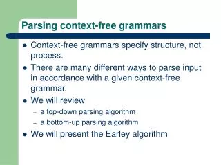
Types of Parsers Use grammars? Grammar-based parsers: CFG, HPSG, … Parsers that do not use grammars explicitly: Ratnaparki’s parser (1997) Require treebanks? Supervised parsers Unsupervised parsers
Where grammars come from: Built by hand Extracted from treebanks Induced from text
BNF Example a (context free) BNF grammar for a simple arithmetic expression. <arithmetic expression>→<term> | <arithmetic expression> + <term> | <arithmetic expression> - <term> <term> → <factor> | <term> x <factor> | <term> / <factor> <factor> → <primary> | <factor> ↑ <primary> <primary> → <variable> | <number> | (<arithmetic expression>) <variable> → <identifier> | <identifier> [<subscript list>] <subscript list> → <arithmetic expression> |<subscript list> , <arithmetic expression>
BNF Example An equivalent (context free) BNF grammar for a simple arithmetic expression. <arithmetic expression → <term> | <arithmetic expression> ↑ <term> | <arithmetic expression> x <term> | <arithmetic expression> + <term> <term> → <primary> | <term> - <primary> | <term> / <primary> <primary> → <variable> | <number> | (<arithmetic expression>) <variable> → <identifier> | <identifier> [<subscript list>] <subscript list> → <arithmetic expression> | <arithmetic expression> , <subscript list>
Parsing Algorithms • Top-down • Bottom-up • Top-down with bottom-up filtering • Earley algorithm • CYK algorithm • ....
Parsing Algorithms - Top Down • Start from the start symbol, and apply rules • Top-down, depth-first, left-to-right parsing • Never explore trees that do not result in S => goal-directed search • Waste time on trees that do not match input sentence.
Parsing Algorithms - Bottom Up • Use the input to guide => data-driven search • Find rules whose right-hand sides match the current nodes. • Waste time on trees that don’t result in S
Parsing Algorithms - Top-down parsing with bottom-up look-ahead filtering Use the input to guide • Both top-down and bottom-up generate too many useless trees. • Combine the two to reduce over-generation • B is a left-corner of A if see handout • Left-corner table provides more efficient look-ahead • Pre-compute all POS that can serve as the leftmost POS in the derivations of each non-terminal category
Dynamic Programming (DP) • DP: • Dividable: The optimal solution of a sub-problem is part of the optimal solution of the whole problem. • Memorization: Solve small problems only once and remember the answers. • Example: T(n) = T(n-1) + T(n-2)
Parsing with DP • Three well-known CFG parsing algorithms: • Earley algorithm (1970) • Cocke-Younger-Kasami (CYK) (1960) • Graham-Harrison-Ruzzo (GHR) (1980)
Earley Algorithm • Use DP to do top-down search • A single left-to-right pass that fills out an array (called a chart) that has N+1 entries. • An entry is a list of states: it represents all partial trees generated so far.
Earley Algorithm - A state A state contains: • A single dotted grammar rule: • [i, j]: • i: where the state begins w.r.t. the input • j: the position of dot w.r.t. the input In order to retrieve parse trees, we need to keep a list of pointers, which point to older states.
Earley Algorithm - Dotted rules 0 Book 1 that 2 flight 3 S --> • VP, [0,0] • S begins position 0 • The dot is at position 0, too. • So, nothing has been covered so far. • We need cover VP next. NP --> Det • Nom, [1,2] • the NP begins at position 1 • the dot is currently at position 2 • so, Det has been successfully covered. • We need to cover Nom next.
Earley Algorithm - Parsing procedure From left to right, for each entry chart[i]: apply one of three operators to each state: • predictor: predictthe expansion • scanner: match input word with the POS after the dot. • completer: advance previous created states.
Earley Algorithm - Predicator • Why this operation: create new states to represent top-down expectations • When to apply: the symbol after the dot is a non-POS. • Ex: S --> NP • VP [i, j] • What to do: Adds new states to current chart: One new state for each expansion of the non-terminal • Ex: VP • V [j, j] VP • V NP [j, j]
Earley Algorithm - Scanner • Why: match the input word with the POS in a rule • When: the symbol after the dot is a POS • Ex: VP --> • V NP [ i, j ], word[ j ] = “book” • What: if matches, adds state to next entry • Ex: V book • [ j, j+1 ]
Earley Algorithm - Completer • Why: parser has discovered a constituent, so we must find and advance states that were waiting for this • When: dot has reached right end of rule • Ex: NP --> Det Nom • [ i, j ] • What: Find every state w/ dot at i and expecting an NP, e.g., VP --> V • NP [ h, i ] • Adds new states to currententry VP V NP • [ h, j ]
Earley Algorithm - Retrieving Parse Trees • Augment the Completer to add pointers to older states from which it advances • To retrieve parse trees, do a recursive retrieval from a complete S in the final chart entry.
Earley Algorithm - Example • Book that flight • Rules: (1) S NP VP (9) N book/cards/flight (2) S VP (10) Det that (3) VP V NP (11) P with (4) VP VP PP (12) V book (5) NP NP PP (6) NP N (7) NP Det N (8) PP P NP
Earley Algorithm - Example • Chart [0], word[0]=book S0: Start .S [0,0] init pred S1: S.NP VP [0,0] S0 pred S2: S .VP [0,0] S0 pred S3: NP.NP PP [0,0] S1 pred S4: NP.Det N [0,0] S1 pred S5: NP.N [0,0] S1 pred S6: VP .V NP [0,0] S2 pred S7: VP .VP PP [0,0] S2 pred
Earley Algorithm - Example • Chart[1], word[1]=that S8: N book . [0,1] S5 scan S9: V book . [0,1] S6 scan S10: NP N. [0, 1] S8 comp [S8] S11: VPV. NP [0,1] S9 comp [S9] S12: S NP. VP [0,1] S10 comp [S10] S13: NPNP. PP [0,1] S10 comp [S10] S14: NP.NP PP [1,1] S11 pred S15: NP.Det N [1,1] S11 pred S16: NP.N [1,1] S11 pred S17: VP.V NP [1,1] S12 pred S18: VP.VP PP [1,1] S12 pred S19: PP.P NP [1,1] S13 pred
Earley Algorithm - Example • Chart[2] word[2]=flight S20: Det that . [1,2] S15 scan S21: NP Det. N [1,2] S20 comp [S20] • Chart[3] S22: Nflight . [2,3] S21 scan S23: NPDet N. [1,3] S22 comp [S20,S22] S24: VP V NP. [0,3] S23 comp [S9,S23] S25: NPNP. PP [1,3] S23 comp [S23] S26: SVP. [0,3] S24 comp [S24] S27: VPVP. PP [0,3] S24 comp [S24] S28: PP.P NP [3,3] S25 pred S29: start S. [0,3] S26 comp [S26]
Earley Algorithm - Retrieving parse trees Start from chart[3], look for start S. [0,3] S26 S24 S9, S23 S20, S22
Earley Algorithm - Summary of Earley algorithm • Top-down search with DP • A single left-to-right pass that fills out a chart • Complexity: A: number of entries: O(N) B: number of states within an entry: O(|G| x N) C: time to process a state: O(|G| x N) O(|G|2 x N3)
Other Concluding Remarks MISSING LINK Man's a kind of Missing Link, fondly thinking he can think..