Parametric Curves
Parametric Curves. 고려대학교 컴퓨터 그래픽스 연구실. Overview. Introduction to mathematical splines Bezier curves Continuity conditions (C 0 , C 1 , C 2 , G 1 , G 2 ) Creating continuous splines C 2 -interpolating splines B-splines Catmull-Rom splines. Introduction.

Parametric Curves
E N D
Presentation Transcript
Parametric Curves 고려대학교 컴퓨터 그래픽스 연구실 cgvr.korea.ac.kr
Overview • Introduction to mathematical splines • Bezier curves • Continuity conditions (C0, C1, C2, G1, G2) • Creating continuous splines • C2-interpolating splines • B-splines • Catmull-Rom splines cgvr.korea.ac.kr
Introduction • Mathematical splines are motivated by the “loftsman’s spline”: • Long, narrow strip of wood or plastic • Used to fit curves through specified data points • Shaped by lead weights called “ducks” • Gives curves that are “smooth” or “fair” • Such splines have been used for designing: • Automobiles • Ship hulls • Aircraft fuselages and wings cgvr.korea.ac.kr
Requirements • Here are some requirements we might like to have in our mathematical splines: • Predictable control • Multiple values • Local control • Versatility • Continuity cgvr.korea.ac.kr
Mathematical Splines • The mathematical splines we’ll use are: • Piecewise • Parametric • Polynomials • Let’s look at each of these terms… cgvr.korea.ac.kr
Parametric Curves • In general, a “parametric” curve in the plane is expressed as: • Example: A circle with radius r centered at the origin is given by: • By contrast, an “implicit” representation of the circle is: cgvr.korea.ac.kr
Parametric Polynomial Curves • A parametric “polynomial” curve is a parametric curve where each function x(t), y(t) is described by a polynomial: • Polynomial curves have certain advantages • Easy to compute • Infinitely differentiable cgvr.korea.ac.kr
Piecewise Parametric Polynomial Curves • A “piecewise” parametric polynomial curve uses different polynomial functions for different parts of the curve • Advantage: Provides flexibility • Problem: How do you guarantee smoothness at the joints? (Problem known as “continuity”) • In the rest parts of this lecture, we’ll look at: • Bezier curves – general class of polynomial curves • Splines – ways of putting these curves together cgvr.korea.ac.kr
Bezier Curves • Developed simultaneously by Bezier (at Renault) and by deCasteljau (at Citroen), circa 1960 • The Bezier Curve Q(u) is defined by nested interpolation: • Vis are “control points” • {V0, …, Vn} is the “control polygon” cgvr.korea.ac.kr
Example: Bezier Curves cgvr.korea.ac.kr
Bezier Curves: Basic Properties • Bezier Curves enjoy some nice properties: • Endpoint interpolation: • Convex hull: The curve is contained in the convex hull of its control polygon • Symmetry: • Q(u) is defined by {V0, …, Vn} ≡ Q(1-u) is defined by {Vn, …, V0} cgvr.korea.ac.kr
Example: 2D Bezier Curves cgvr.korea.ac.kr
Bezier Curves: Explicit Formulation • Let’s give Vi a superscript Vij to indicate the level of nesting • An explicit formulation Q(u) is given by the recurrence: cgvr.korea.ac.kr
is the i ‘th Bernstein polynomial of degree n Explicit Formulation (cont.) • For n=2, we have: • In general: cgvr.korea.ac.kr
Example: Explicit Formulation cgvr.korea.ac.kr
Bezier Curves: More Properties • Here are some more properties of Bezier curves • Degree: Q(u) is a polynomial of degree n • Control points: How many conditions must we specify to uniquely determine a Bezier curve of degree n cgvr.korea.ac.kr
More Properties (cont.) • Tangent: • k ‘th derivatives: In general, • Q(k)(0) depends only on V0, …, Vk • Q(k)(1) depends only on Vn, …, Vn-k • At intermediate points , all control points are involved every derivative cgvr.korea.ac.kr
Explanation cgvr.korea.ac.kr
Cubic Curves • For the rest of this discussion, we’ll restrict ourselves to piecewise cubic curves • In CAGD, higher-order curves are often used • Gives more freedom in design • Can provide higher degree of continuity between pieces • For Graphics, piecewise cubic lets you do about anything • Lowest degree for specifying points to interpolate and tangents • Lowest degree for specifying curve in space • All the ideas here generalize to higher-order curves cgvr.korea.ac.kr
Matrix Form of Bezier Curves • Bezier curves can also be described in matrix form: cgvr.korea.ac.kr
Display: Recursive Subdivision • Q: Suppose you wanted to draw one of these Bezier curves – how would you do it? • A: Recursive subdivision cgvr.korea.ac.kr
Display (cont.) • Here’s pseudo code for the recursive subdivision display algorithm • ProcedureDisplay({V0, …, Vn}) • if {V0, …, Vn} flat within e then • Output line segment V0Vn • else • Subdivide to produce {L0, …, Ln} and {R0, …, Rn} • Display({L0, …, Ln}) • Display({R0, …, Rn}) • end if • end procedure cgvr.korea.ac.kr
Splines • To build up more complex curves, we can piece together different Bezier curves to make “splines” • For example, we can get: • Positional (C0) Continuity: • Derivative (C1) Continuity: • Q: How would you build an interactive system to satisfy these conditions? cgvr.korea.ac.kr
Advantages of Splines • Advantages of splines over higher-order Bezier curves: • Numerically more stable • Easier to compute • Fewer bumps and wiggles cgvr.korea.ac.kr
Tangent (G1) Continuity • Q: Suppose the tangents were in opposite directions but not of same magnitude – how does the curves appear? • This construction gives “tangent (G1) continuity” • Q: How is G1 continuity different from C1? cgvr.korea.ac.kr
Qn+1(u) Qn+1(u) Qn+1(u) Explanation • Positional (C0) continuity • Derivative (C1) continuity • Tangent (G1) continuity Qn(u) Qn(u) Qn(u) cgvr.korea.ac.kr
Curvature (C2) Continuity • Q: Suppose you want even higher degrees of continuity – e.g., not just slopes but curvatures – what additional geometric constraints are imposed? • We’ll begin by developing some more mathematics..... cgvr.korea.ac.kr
Operator Calculus • Let’s use a tool known as “operator calculus” • Define the operator D by: • Rewriting our explicit formulation in this notation gives: • Applying the binomial theorem gives: cgvr.korea.ac.kr
Taking the Derivative • One advantage of this form is that now we can take the derivative: • What’s (D-1)V0? • Plugging in and expanding: • This gives us a general expression for the derivative Q’(u) cgvr.korea.ac.kr
W0 Q’(1) Q’(0) W1 W2 W3 Specializing to n=3 • What’s the derivative Q’(u) for a cubic Bezier curve? • Note that: • When u=0: Q’(u) = 3(V1-V0) • When u=1: Q’(u) = 3(V3-V2) • Geometric interpretation: • So for C1 continuity, we need to set: V0 V1 V2 V3 cgvr.korea.ac.kr
Taking the Second Derivative • Taking the derivative once again yields: • What does (D-1)2 do? cgvr.korea.ac.kr
Q’’(0) Q’’(1) Q’(0) Q’(1) Second-Order Continuity • So the conditions for second-order continuity are: • Putting these together gives: • Geometric interpretation V0 V1 V3 V2 cgvr.korea.ac.kr
C3 Continuity V0 V3 V1 V2 cgvr.korea.ac.kr
C3 Continuity W1 W2 W3 V0 V3 W0 V1 V2 cgvr.korea.ac.kr
C3 Continuity W1 W2 W0 W3 V0 V3 V1 V2 cgvr.korea.ac.kr
C3 Continuity W2 W1 W0 W3 V0 V3 V1 V2 cgvr.korea.ac.kr
C3 Continuity W2 W3 W1 W0 V0 V3 V1 V2 cgvr.korea.ac.kr
C3 Continuity • Summary of continuity conditions • C0 straightforward, but generally not enough • C3 is too constrained (with cubics) W2 W3 W1 W0 V0 V3 V1 V2 cgvr.korea.ac.kr
Creating Continuous Splines • We’ll look at three ways to specify splines with C1 and C2 continuity • C2 interpolating splines • B-splines • Catmull-Rom splines cgvr.korea.ac.kr
C2 Interpolating Splines • The control points specified by the user, called “joints”, are interpolated by the spline • For each of x and y, we needed to specify 3 conditions for each cubic Bezier segment. • So if there are m segments, we’ll need 3m-1 conditions • Q: How many these constraints are determined by each joint? joint cgvr.korea.ac.kr
In-Depth Analysis • At each interior joint j, we have: • Last curve ends at j • Next curve begins at j • Tangents of two curves at j are equal • Curvature of two curves at j are equal • The m segments give: • m-1 interior joints • 3 conditions • The 2 end joints give 2 further constraints: • First curve begins at first joint • Last curve ends at last joint • Gives 3m-1 constraints altogether cgvr.korea.ac.kr
End Conditions • The analysis shows that specifying m+1 joints for m segments leaves 2 extra degree of freedom • These 2 extra constraints can be specified in a variety of ways: • An interactive system • Constraints specified as user inputs • “Natural” cubic splines • Second derivatives at endpoints defined to be 0 • Maximal continuity • Require C3 continuity between first and last pairs of curves cgvr.korea.ac.kr
C2 Interpolating Splines • Problem: Describe an interactive system for specifying C2 interpolating splines • Solution: 1. Let user specify first four Bezier control points 2. This constraints next 2 control points – draw these in. 3. User then picks 1 more 4. Repeat steps 2-3. cgvr.korea.ac.kr
Global vs. Local Control • These C2 interpolating splines yield only “global control” – moving any one joint (or control point) changes the entire curve! • Global control is problematic: • Makes splines difficult to design • Makes incremental display inefficient • There’s a fix, but nothing comes for free. Two choices: • B-splines • Keep C2 continuity • Give up interpolation • Catmull-Rom Splines • Keep interpolation • Give up C2 continuity – provides C1 only cgvr.korea.ac.kr
B-Splines • Previous construction (C2 interpolating splines): • Choose joints, constrained by the “A-frames” • New construction (B-splines): • Choose points on A-frames • Let these determine the rest of Bezier control points and joints • The B-splines I’ll describe are known more precisely as “uniform B-splines” cgvr.korea.ac.kr
V2 V2 V1 V3 V0 Explanation • C2 interpolating spline • B-splines V1 V0 B2 B1 B0 B3 cgvr.korea.ac.kr
n+1 control points polynomials of degree d-1 B-Spline Construction cgvr.korea.ac.kr
n+1 control points polynomials of degree d-1 B-Spline Construction • The points specified by the user in this construction are called “deBoor points” cgvr.korea.ac.kr
B-Spline Properties • Here are some properties of B-splines: • C2 continuity • Approximating • Does not interpolate deBoor points • Locality • Each segment determined by 4 deBoor points • Each deBoor point determine 4 segments • Convex hull • Curves lies inside convex hull of deBoor points cgvr.korea.ac.kr
Algebraic Construction of B-Splines • V1 = (1 - 1/3)B1 + 1/3 B2 • V2 = (1- 2/3)B1 + 2/3 B2 • V0 = ½ [(1- 2/3)B0 + 2/3 B1] + ½ [(1 - 1/3)B1 + 1/3 B2] = 1/6 B0 + 2/3 B1 + 1/6 B2 • V3 = 1/6 B1 + 2/3 B2 + 1/6 B3 cgvr.korea.ac.kr