Download

1 / 47
470 likes | 666 Vues
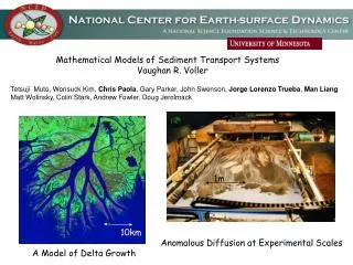
Mathematical Models of Sediment Transport Systems Vaughan R. Voller . Tetsuji Muto, Wonsuck Kim, Chris Paola , Gary Parker, John Swenson, Jorge Lorenzo Trueba , Man Liang Matt Wolinsky, Colin Stark, Andrew Fowler, Doug Jerolmack . 1m. 10km.

E N D
Mathematical Models of Sediment Transport Systems Vaughan R. Voller Tetsuji Muto, Wonsuck Kim, Chris Paola, Gary Parker, John Swenson, Jorge Lorenzo Trueba, Man Liang Matt Wolinsky, Colin Stark, Andrew Fowler, Doug Jerolmack 1m 10km Anomalous Diffusion at Experimental Scales A Model of Delta Growth
Bangladesh Katrina
The Disappearing Mississippi Delta—Motivation Provided by Wonsuck Kim et al, EOS Aug 2009 New Orleans Due to – Upstream Damming (limiting sediment supply) Artificial Channelization of the river (limiting flooding) Increased subsidence (?) creating off shore space that needs to be filled Bird’s foot Each year Louisiana loses ~44 sq k of costal wetlands Loss of a buffer that could protect inland infrastructure
A plan is on the table to reverse this trend is to create breaks in the levees to allow for flooding, sediment deposit, and land growth Costly and Risky: Is there enough sediment? Will it be sustainable ? How long will it take ?
A lucky accidental natural experiment New Orleans Some 100 k or so to the West of New-Orleans ,in the 1970’s a navigation channel was created on a tributary of the Mississippi. This resulted in a massive sediment diversion and over the next 30 years the building of an delta ~20K in dimension ~20k Wax-Lake Delta
Can the experience of Wax Lake be transported to the Bird’s Foot? Sediment Delta Growth Models developed can be validated with Wax Lake data? Graphic by Wonsuck Kim, UAT Building Delta Models is achieved by appealing to heat and mass transfer analogies
Examples of Sediment Deltas Water and sediment input Sediment Fans 1km
The delta shoreline is a moving boundary Advanced in time due to sediment input Land profile view Water advancing shore-line land water sediment flux
A One D Experiment mimicking building of delta profile, Tetsuji Muto and Wonsuck Kim Sediment and Water Mix introduced into a slot flume (2cm thick) with a fixed Sloping bottom and fixed water depth shore-line moves in response to sediment input Maintains a constant submarine slope Can we construct a model for this ?
In a Laboratory setting with constant flow discharge and shallow depth d(epth) Drag + Momentum Balance And when coupled to the Sediment Transport Law (assuming bed shear >> Sheild’s stress)
The Swenson Analogy—Melting and Shoreline Movement Water and Sediment line discharges Shore-line Advance no subsidence or sea-level change Latent heat increases in space Stefan Melting Problem T Shore-line condition
Apply this analogy to experiments JORGE LORENZO-TRUEBA1, VAUGHAN R. VOLLER, TETSUJI MUTO ,WONSUCK KIM, CHRIS PAOLA AND JOHN B. SWENSON J. Fluid Mech. (2009), vol. 628, pp. 427–443 Provide sediment line-flux mm2/s water line-discharge mm2/s
At capacity transport Governing Equations fixed basement Note: Two moving boundaries moving in opposite directions. (1) shoreline, (2) bed-rock/alluvial transition (point on basement where sediment first deposits ) Four Boundary Conditions Are Needed
A closed form similarity solution for tracking fronts is found Slope Ratio Where the lambdas are functions of the dimensionless variables the slope ratio R and
predicted fluvial surface Experiment vs. Analytical: VALIDATION J. Fluid Mech. (2009), vol. 628, pp. 427–443 experimental analytical Get fit by choosing diffusivity from Geometric measurements From one exp. snap-shot
High R lower R In field setting Value of slope ratio R controls “sensitivity” of fronts J. Fluid Mech. (2009), vol. 628, pp. 427–443
Common Field observation Lower than expected curvature for fluvial surface experimental analytical
In a Laboratory setting with constant flow discharge and shallow depth d(epth) Drag Momentum Balance And when coupled to the sediment transport law (assuming bed shear >> Sheild’s stress) Suggests a non-linear diffusive model
Non-Linear diffusion model J. Lorenzo-Trueba, V.R. Voller J. Math. Anal. Appl. 366 (2010) 538–549 also has sim. sol but requires numerical solution Closed form only when geometric wedge
Linear Geometric J. Lorenzo-Trueba, V.R. Voller J. Math. Anal. Appl. 366 (2010) 538–549 Not until you reach high values of R do you see any real difference R
Back to lack of curvature in Experiments ~3m “Jurasic Tank” Experiment at close to steady state Diffusion solution “too-curved” subsidence
Exp. Model ~3m Heterogeneity occurs at all scales Up to an including the domain. REV can not be identified Volume over which average properties can be applied globally. Is this equation valid Clear separation between scale of heterogeneity and domain. An REV can be identified Not a slot
Exp Model x Transport controlled by Non-local “events” suggesting --- path-dependence described through hereditary integrals Non-Gaussian behaviors with “thick” power-law tails allowing for occurrence of extreme events Through use of volume averaging generic Advection-Diffusion transport equation will have form Processes that can be embodied into a fractional Advection-Diffusion Equation (fADE) fractional flux depends on weighted average of non-local slopes (up and down stream)
First we take a pragmatic approach and investigate what happens if we replace the diffusion flux with a fractional flux Will this reduce curvature ? A toy problem is introduced [area/time] solution [length/s] Piston subsidence of base
Note Solution First we will just blindly try a pragmatic approach where we will write down a Fractional derivative from of our test problem, solve it and compare the curvatures. Our first attempt is based on the left hand Caputo derivative With LOOKS UPSTREAM The divergence of a non-local fractional flux
Clearly Not a good solution expected predicted
Our second attempt is based on the right hand Caputo derivative With LOOKS DOWN-STREAM Note Solution On [0,1]
Right-Hand Caputo Looks like this Has “correct behavior” When we scale to The experimental setup We get a good match
And when a fraction flux is used it can match the observed lack of curvature Voller and Paola JGR (to appear) Right
But the question remains Is this physically meaningful ?
The movement of the red particle is controlled by the movement of the green particle at the chain head –a movement controlled by the slope at the green particle x side view 1 plan view A simple minded model: Down stream conditions influence upstream transport Imagine that particles transport through system as chains The lengths of the chains vary and can take values up to the length of the system So at a given cross section x we can write down a the flux as a weighted average of the down-stream slopes
If we choose power law-weights And take limit as With change in variable With simple mined particle chain model Flux ix given by the Right-Hand Caputo
Fractional diffusion can predict observed low curvature A simple minded model can provide a physical rational for fractional model based on down stream control of flux Basic diffusion models can lead to interesting math and reproduce experiments
Nright Nleft Shown How classic numerical heat transfer (enthalpy method) can be used to model key geoscince problem Illustrated how a Monte-Carlo Solution based on a Levy PDF Can solve fractional BVP
Comparison of Monte-Carlo and analytical CLAIM: If steps are chosen from a Levy distribution Maximum negative skew, This numerical approach will also recover Solutions to Suggest that Monte Carlo Associated with a PDF Could resolve multiple situations
A Monte Carlo Solution CLAIM: If steps are chosen from a Levy distribution Maximum negative skew, This numerical approach will also recover Solutions to Well know (and somewhat trivial) that a Monte Carlo simulation originating from a ‘point’ and using steps from a normal distribution will after multiple realizations recover the temperature at the ‘point’ Nright Nleft Tpoint = fraction of walks that exit on Left
If the fractional derivative is identified as a Caputo derivative (there are a number of reasonable definitions) then the closed solution is As a demonstration of one-way we may go-about solving such systems let us Consider the example fractional BVP This is a steady state problem in which the left hand side represents a Local balance of a Non-Local flux
time scale for such a process Anomalous: Super-Diffusion ~3m On using results from “fractal” methods a scale independent model can be posed in terms of a fractional derivative Related to a Levy PDF distribution It has “Fat Tails” Extreme events have finite probability Such considerations could be important in micro-scale heat transfer-where the required resolution is close the scale of the mechanisms in the heat conduction Process.
BUT On a land surface, spatial and temporal variations are at an “observable scale” –at or close to the scale of resolution Observed -Holdup-release events -History dependent fluxes ~3m Monte Carlo Calculation of Fractional Heat Conduction As noted above the transport of sediment (flux volume/area-time) can be described by A “diffusion” like law
~3m BUT On a land surface, spatial and temporal variations are at an “observable scale” This is similar to situation in a porous media—where it is known that length scale of resolution where the hydraulic Conductivity has a power law dependence with the scale at which it is resolved. Modeling a reservoir at scale using a hydraulic conductivity determined at a scale Will result in under prediction of transport
For field condition then plot of solution vs. R= observed range R Errors appears when slope ratio is high A thin wedge at on-lap
Verification: Comparison of numerical and analytical predictions VERIFY Numerical Approach Approximation Assumptions Numerical Solution Phenomenological Assumptions Model Limit Case Assumptions Physical Process Analytical Solution Validation: If assumptions for Analytical solution are consistent with Physical assumptions In experiment Can VALIDATE phenomenological assumptions Isolate Key Phenomena Experiment The Modeling Paradigm