Sorting
Sorting. Sorting includes internal sorting and external sorting Internal sorting : the entire sort can be done in main memory, i.e., all elements needed to be sorted can be stored entirely in main memory.

Sorting
E N D
Presentation Transcript
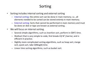
Sorting • Sorting includes internal sorting and external sorting • Internal sorting: the entire sort can be done in main memory, i.e., all elements needed to be sorted can be stored entirely in main memory. • External sorting: Sorts that cannot be performed in main memory and must be done on disk or tape are known as external sorting. • We will focus on internal sorting. • Several simple algorithms, such as insertion sort, perform in O(N2) time. • Shellsort that is very simple to code, first breaks ( N2 ) barrier, and is efficient in practice. • Slightly more complicated sorting algorithms, such as heap sort, merge sort, quick sort, take O(NlogN) time. • Linear time sorting algorithms, such as bucket sort.
Preliminaries The efficiency of data handling can often be substantially increased if the data are sorted according to some criteria of order. We assume: • The objects being sorted are elements of an array. • The objects being sorted are of type Comparable, which is just a synonym for whatever class of object we wish to place in the array. • If necessary, the Comparable class overloads the standard C++ operators =, > and < that used by the sort algorithms. That is, = is used for copying elements, while > and < compare two elements with respect to the defined criteria. This enables sort criteria to vary from one element type to another.
Insertion Sort • Insertion sort is one of the simplest sorting algorithms. • The algorithm • Insertion sort consists of N-1 passes. • For pass p = 1 through N-1, insertion sort ensures that the elements in positions 0 through p are in sorted order. • Insertion sort makes use of the fact that elements in positions 0 through p-1 are already known to be in sorted order, and move the element in position p left until its correct place is found among the first p+1 elements.
Insertion Sort Examples • Sort 34, 8, 64, 51, 32, and 21 position: 0 1 2 3 4 5 34 8 64 51 32 21 First pass: 348 64 51 32 21 p = 1 8 34 64 51 32 21 second pass: 8 3464 51 32 21 p = 2 8 3464 51 32 21 third pass: 8 346451 32 21 p = 3 8 345164 32 21 8 345164 32 21 fourth pass: 8 34516432 21 p = 4 8 34513264 21 8 34325164 21 8 32345164 21 8 32345164 21
Insertion Sort Examples • Sort 34, 8, 64, 51, 32, and 21 (cont.) position: 0 1 2 3 4 5 fifth pass: 8 3234516421 p = 5 8 3234512164 8 3234215164 8 3221 345164 8 2132345164 8 2132345164
Insertion Sort C++ code template <class comparable> void InsertionSort (vector<comparable> & a) { int j; for (int p=1; p < a. size( ); p++) // perform N-1 passes { // for each iteration p, a[0 .. p-1] in sorted order. comparable tmp = a[p]; for (j = p; j > 0 && tmp < a[j-1]; j--) a[j] = a[j-1]; a[j] = tmp; } } move the element in position p left until its correct place is found among the first p+1 elements. 8 346451 32 21 p j
Insertion Sort Performance • InsertionSort() includes two nested loops. • The inner loop can be executed at most p+1 times for each value of p. • p iterates from 1 to N-1 • The number of iterations of the inner loop is given by: 2+3+ … +N = N(N+1)/2 - 1 • The running time of InsertionSort is O(N2).
Insertion Sort Best Cases • If the input data elements are in increasing order, the inner loop is terminated immediately and thus the running time is O(N). • For example: sort 8 21 32 34 51 64 position: 0 1 2 3 4 5 8 21 32 34 51 64 First pass: 821 32 34 51 64 p = 1 821 32 34 51 64 second pass: 82132 34 51 64 p = 2 821 32 34 51 64 third pass: 821 3234 51 64 p = 3 821 32 34 51 64 fourth pass: 821 32 3451 64 p = 4 8 21 32 34 51 64 fifth pass: 8 21 32 34 5164 p = 5 821 32 3451 64
Insertion Sort Worst Cases • If the input data elements are in decreasing order, the inner loop is executed p+1 times for each value of p and thus the running time is O(N2). • For example: sort 64 51 34 32 21 8 position: 0 1 2 3 4 5 64 51 34 32 21 8 fourth pass: 32 34 51 64 218 j=4 p = 4 32 34 51 21 64 8 j=3 32 34 21 51 64 8 j=2 32 21 34 51 64 8 j=1 21 32 34 51 64 8 j=0 21 32 34 51 64 8
Shellsort • Shellsort was one of the first algorithms to break the quadratic barrier. • Shellsort works by comparing elements that are distant; the distance between comparisons decreases as the algorithm runs until the last phase, in which adjacent elements are compared. • Basic ideas • Choose a sequence, h1=1, h2, …, ht, called the increment sequence. • For each hk = ht , …, h2, h1, sort all elements spaced hk apart. (After a phase, using some increment hk, for every i, we have a[i] <= a[i+hk]; all elements spaced hk apart are in sorted order. The file is then said to be hk-sorted.) • In each phase, use insertion sort to sort all elements spaced hk apart. For example, Original: 809360124230688510 after 3-sort: 124210688530809360
Shellsort Example Suppose we have an array containing the following integers: 80 93 60 12 42 30 68 85 10 • Choose {3, 2, 1} as the increment sequence. • For each hk = 3, 2, 1, sort all elements spaced hk apart using insertion sort. • For hk = 3, divide the original array into three segments (all elements in each segment are spaced hk apart in the original array). 80 12 68 segment 1 93 42 85 segment 2 60 30 10 segment 3 (809360124230688510) and sort each segment using insertion sort: 12 68 80 42 85 93 10 30 60 The original array, partially sorted, now appears as 124210688530809360
Shellsort Example • For each hk = 3, 2, 1, sort all elements spaced hk apart using insertion sort. (After 3-sort: 12 42 10 68 85 30 80 93 60) • For hk = 2, divide the 3-sorted array into two segments (all elements in each segment are spaced hk apart in the 3-sorted array). 12 10 85 80 60 segment 1 42 68 30 93 segment 2 (124210688530809360) and sort each segment using insertion sort: 10 12 60 80 85 30 42 68 93 The array takes the form: 10 30 12 42 60 68 80 93 85 (after 2-sort) • For hk = 1, sort the 2-sorted array using insertion sort. 10 12 30 42 60 68 80 85 93
How to Choose the Increment Sequence • Any increment sequence will do as long as h1 = 1, but some choices are better than others. • Shell’s increments: ht = N/2 and hk = hk+1/2 Ex. N = 9: 1, 2, 4 N = 21: 1, 2, 5, 10 • Hibbard’s increments: 1, 3, 7, …, 2k-1 (such that 2k-1 <= N and 2k+1-1 > N) Ex. N = 9: 1, 3, 7 N = 21: 1, 3, 7, 15 • Sedgewick’s increments: 1, 5, 19, 41, 109 …, in which the terms are either of the form 9*4i-9*2i+1 or 4i-3*2i+1. Ex. N = 9: 1, 5 N = 21: 1, 5, 19
C++ code for Shellsort /** * Shellsort, using Shell’s (poor) increments. */ template <class Comparable> void shellsort( vector<Comparable> & a ) { int j; for ( int gap = a.size() / 2; gap > 0; gap /= 2 ) for ( int i = gap; i < a.size(); i ++) { Comparable tmp = a[ i ]; for ( j = i; j >= gap && tmp < a[ j – gap ]; j -= gap ) a [j ] = a[ j – gap ]; a [ j ] = tmp; } } //Shell’s increments Use insertion sort to sort elements in each segments in sorted order. That is, for each position, i, in gap, gap+1, …, N-1, place the element in the correct spot among i, i-gap, i-2*gap, i-3*gap, …, etc.
i i i i i i i i i i Shellsort Using Shell’s Increments - Example Original : 81 99 11 96 12 98 17 95 gap = 4 : 81 991196 12 981795 81 991196 12 981795 12 991196 81 981795 12 981196 81 991795 12 981196 81 991795 12 981195 81 991796 Place the element at i in the the correct spot among the elements in the same segment and at the positions before i. gap = 2 : 12 98 11 95 81 99 17 96 11 98 12 95 81 99 17 96 11 98 12 95 81 99 17 96 11 95 12 98 81 99 17 96 11 95 12 98 81 99 17 96 11 95 12 98 81 99 17 96 11 95 12 98 17 99 81 96 11 95 12 96 17 98 81 99
Shellsort Running Time • The running time of Shellsort depends on the choice of increment sequence. • The worst-case running time of Shellsort, using Shell’s increments, is O(N2). • The worst-case running time of Shellsort using Hibbard’s increments is O(N3/2). • The worst-case running time of Shellsort using Sedgewick’s increments is O(N4/3). • The average-case running time of Shellsort, using Hibbard’s increments, is thought to be O(N5/4), based on simulations, but nobody has been able to prove this. • The average running time is conjectured to be O(N7/6).
Heapsort • Binary heaps can be used to sort in O(NlogN) time. • Basic ideas • Step 1: Build a binary heap of N elements • Step 2: Remove the root and reheap (perform the deleteMin operation) • Step 3: Repeat step 2 until empty.
58 59 53 59 26 41 58 97 26 41 31 53 31 97 Binary heaps (review) • What is a binary heap? • Complete binary tree: a binary tree that is completely filled, with the possible exception of the bottom level, which is filled from left to right. • Heap-order property: for every node x, the key in the parent of x is smaller than (or equal to) the key in x, with the exception of the root. • How to build a binary heap for N elements? • build a complete binary tree first ignore the heap-order property at the moment • apply percolate-down for each node starting at the last non-leaf node. 41 31 53 97 58 59 26 53 59 26 41 58 31 97 1 2 3 4 5 6 7 8 9 10 0 1 2 3 4 5 6 7 8 9 10 0
97 26 59 97 53 41 59 58 97 53 41 41 53 31 41 59 58 97 53 31 58 Binary heaps (review) • deleteMin: • Remove the element in the root and create a hole in the root. • Percolate the hole down so that the last element in the heap can be placed in the hole. 41 31 53 97 58 59 26 41 31 53 97 58 59 1 2 3 4 5 6 7 8 9 10 0 1 2 3 4 5 6 7 8 9 10 0 31 31 58 59 41 53 97 58 59 31 41 58 53 97 59 31 1 2 3 4 5 6 7 8 9 10 0 1 2 3 4 5 6 7 8 9 10 0
41 53 97 59 58 97 53 31 41 26 Heapsort Example Sort 97 53 59 26 41 58 31 • Build a binary heap for 97 53 59 26 41 58 31 • Remove root 26 and reheap: 41 31 53 97 58 59 26 1 2 3 4 5 6 7 0 31 58 59 26 41 58 53 97 59 31 1 2 3 4 5 6 7 0 1 2 3 4 5 6 7 0
59 59 97 97 53 Heapsort Example Sort 97 53 59 26 41 58 31 • Remove root 31 and reheap: • Remove root 41 and reheap: 41 58 26 31 53 58 59 97 41 1 2 3 4 5 6 7 0 1 2 3 4 5 6 7 0 53 58 26 31 41 59 58 97 53 1 2 3 4 5 6 7 0 1 2 3 4 5 6 7 0
59 Heapsort Example Sort 97 53 59 26 41 58 31 • Remove root 53 and reheap: • Remove root 58 and reheap: 58 97 53 26 31 41 59 97 58 1 2 3 4 5 6 7 0 1 2 3 4 5 6 7 0 59 97 53 26 31 41 58 97 59 1 2 3 4 5 6 7 0 1 2 3 4 5 6 7 0
Heapsort Example Sort 97 53 59 26 41 58 31 • Remove root 59 and reheap: • Remove root 97: 97 53 26 58 59 31 41 97 1 2 3 4 5 6 7 0 1 2 3 4 5 6 7 0 59 97 53 26 31 41 58 1 2 3 4 5 6 7 0 1 2 3 4 5 6 7 0
Heapsort Running Time • To build a binary heap takes O(N) time. • Performing N deleteMin operations takes O(NlogN) time. • Total running time is O(NlogN). • Drawback: need to use an extra array.
97 53 41 97 53 41 Heapsort Improving Space Efficiency • A clever way to avoid using a second array makes use of the fact that after each deleteMin, the heap shrinks by 1. • The cell that was last in the heap can be used to store the element that was just deleted. 31 58 After remove the smallest element 26. 59 26 41 58 53 97 59 31 1 2 3 4 5 6 7 0 1 2 3 4 5 6 7 0 31 58 59 26 41 58 53 97 59 31 1 2 3 4 5 6 7 0
59 97 53 31 41 26 58 97 53 41 Improving Space Efficiency Example Sort 97 53 59 26 41 58 31 • Build a binary heap for 97 53 59 26 41 58 31 • Remove root 26 and reheap: 41 31 53 97 58 59 26 1 2 3 4 5 6 7 0 31 58 59 26 41 58 53 97 59 31 1 2 3 4 5 6 7 0
59 97 97 59 53 Improving Space Efficiency Example Sort 97 53 59 26 41 58 31 • Remove root 31 and reheap: • Remove root 41 and reheap: 41 58 26 31 53 58 59 97 41 1 2 3 4 5 6 7 0 53 58 26 41 59 58 97 53 31 1 2 3 4 5 6 7 0
97 59 Improving Space Efficiency Example Sort 97 53 59 26 41 58 31 • Remove root 53 and reheap: • Remove root 58 and reheap: 58 97 31 41 26 59 97 53 58 1 2 3 4 5 6 7 0 59 26 31 41 97 58 59 53 1 2 3 4 5 6 7 0
Improving Space Efficiency Example Sort 97 53 59 26 41 58 31 • Remove root 59 and reheap: • Remove root 97 and reheap: 97 26 31 41 59 58 97 53 1 2 3 4 5 6 7 0 26 31 41 59 58 97 53 • The resulting array contains the elements in decreasing sorted order. • If we want the elements in the more typical increasing sorted order, how to solve? 1 2 3 4 5 6 7 0
(max)Heap • In the original heap, the parent has a smaller element than its children. • (max)Heap • A complete binary tree • Heap order property: for every node x, the key in the parent of x is larger than (or equal to) the key in x, with the exception of the root.
31 41 26 59 53 97 58 41 26 53 Heapsort Using (max)Heap Example Sort 97 53 59 26 41 58 31 • Build a (max)heap for 97 53 59 26 41 58 31 • Remove root 97 and reheap: 53 59 26 41 58 31 97 1 2 3 4 5 6 7 0 59 58 31 97 53 58 26 41 31 59 1 2 3 4 5 6 7 0
41 26 53 26 41 Heapsort Using (max)Heap Example Sort 97 53 59 26 41 58 31 • Remove root 59 and reheap: • Remove root 58 and reheap: 58 31 97 53 31 26 41 59 58 1 2 3 4 5 6 7 0 53 31 97 41 31 26 58 59 53 1 2 3 4 5 6 7 0
26 26 Heapsort Using (max)Heap Example Sort 97 53 59 26 41 58 31 • Remove root 53 and reheap: • Remove root 41 and reheap: 41 31 97 26 31 53 58 59 41 1 2 3 4 5 6 7 0 31 97 26 41 53 58 59 31 1 2 3 4 5 6 7 0
Heapsort Using (max)Heap Example Sort 97 53 59 26 41 58 31 • Remove root 31 and reheap: • Remove root 26 and reheap: 26 97 31 41 53 58 59 26 1 2 3 4 5 6 7 0 97 31 41 53 58 59 26 1 2 3 4 5 6 7 0
Mergesort • Mergesort runs in O(NlogN) worst-case running time. • The number of comparisons used is nearly optimal. • Mergesort is a fine example of a recursive algorithm. • We give two implementations: recursive one and non-recursive one.
Actr Bctr Cctr Merging Two Sorted Lists • The fundamental operation in this algorithm is merging two sorted lists. • Basic ideas • Takes two input arrays A and B in sorted order, and an output array C. • Three counters, Actr, Bctr, and Cctr, which are initially set to the beginning of their respective arrays. • The smaller of A[Actr] and B[Bctr] is copied to the next entry in C (i.e., C[Cctr]), and the appropriate counters are advanced. • When either input list is exhausted, the remainder of the other list is copied to C. A B C 24 26 13 27 38 1 15 2
A B C 1 24 26 13 27 38 15 2 A B C 1 24 26 13 27 38 1 15 2 A B C 1 24 26 13 27 38 1 15 2 2 A B C 1 24 26 13 27 38 1 15 2 2 13 Cctr Bctr Actr Cctr Actr Bctr Bctr Actr Bctr Cctr Actr Cctr Merging Two Sorted Lists Example • Suppose we want to merge array A containing 1, 13, 24, 26, and array B containing 2, 15, 27, 38 1 2 13 15
A B C 1 24 26 13 27 38 1 15 2 2 13 15 A B C 1 24 26 13 27 38 1 15 2 2 13 24 15 A B C 1 24 26 13 27 38 1 15 2 2 13 24 26 15 A B C 1 24 26 13 27 38 1 15 2 2 13 24 26 27 38 15 Cctr Bctr Actr Actr Bctr Bctr Actr Cctr Bctr Actr Cctr Cctr Merging Two Sorted Lists Example • Suppose we want to merge array A containing 1, 13, 24, 26, and array B containing 2, 15, 27, 38 (cont.) 24 26 Now the array A is exhausted. Then the remainder of the array B is copied to C
rightPos rightEnd leftPos Merging Two Sorted Lists C++ Code B A a leftEnd points to the last position of subarray A; tmpPos is the next available position in array tmpArray to place the merged result. One pass traversal of A and B; make sure not to go Beyond the end position of A or B. If current element in A is no larger than current element In B, place the current element in A into tmpArray, and advance leftPos and tmpPos by one. If we exhaust array B, copy the remainder of array A to tmpArray. If we exhaust array A, copy the remainder of array B to tmpArray.
Recursive Mergesort • The basic idea • If N = 1, there is only one element to sort, and the answer is at hand. • Otherwise, • Recursively mergesort the first half; • Recursively mergesort the second half; • This gives two sorted halves, which can then be merged together using the merging algorithm. • For instance, suppose to sort the eight-element array 24 13 26 1 2 27 38 15 • Recursively sort the first four elements: 24 13 26 1 1 13 24 16 • Recursively sort the second four elements: 2 27 38 15 2 15 27 38 • Merge the two halves 1 2 13 15 24 26 27 38
Recursive Mergesort C++ Code … … a center left right
1 2 13 15 24 26 27 38 mS(a, 0, 7) 24 13 26 1 2 27 38 15 2 15 27 38 1 13 24 26 mS(a, 4, 7) mS(a, 0, 3) 24 13 26 1 2 27 38 15 1 26 15 38 13 24 2 27 mS(a, 4, 5) mS(a, 0, 1) mS(a, 2, 3) mS(a, 6, 7) 26 1 2 27 38 15 24 13 mS(a, 7, 7) mS(a, 3, 3) mS(a, 2, 2) mS(a, 6, 6) mS(a, 0, 0) mS(a, 4, 4) mS(a, 1, 1) mS(a, 5, 5) 27 15 2 1 13 38 26 24 Execution of the Recursive mergeSort 7 0 1 3 4 2 5 6 a 13 26 2 27 38 15 24 1 • Suppose to sort the following integers 38 26 15 1 27 2 13 24
Divide-and-Conquer • mergeSort is a classic devide-and-conquer strategy. • Basic ideas: Break the problem into several subproblems that are similar to the original problem but smaller in size, solve the subproblems recursively, and then combine these solutions to create a solution to the original problem. • The divide-and-conquer paradigm involves three steps at each level of the recursion: • Divide the problem into a number of subproblems. • Conquer the subproblems by solving them recursively. If the subproblems sizes are small enough, however, just solve the subproblems in a straightforward manner. • Combine the solutions to the subproblems into the solution for the original problem.
1 2 2 3 4 5 6 6 1 3 2 6 5 2 4 6 1 2 3 6 2 4 5 6 4 6 1 3 2 6 5 2 4 6 1 3 2 6 2 5 2 4 6 1 3 2 6 5 2 4 6 1 3 2 6 5 Divide-and-Conquer mergeSort • The merge sort algorithm closely follows the divide-and-conquer paradigm. • Divide: Divide the n-element array to be sorted into two subarrays of n/2 elements each. • Conquer: Sort the two subarrays recursively using mergeSort. • Combine: Merge the two sorted subarrays to produce the sorted answer. 5 2 4 6 1 3 2 6
Analysis of mergeSort • mergeSort works correctly when the number of elements is not even. • Our analysis is simplified. We assume that the original problem size is a power of two, so that we always split into even halves. • Assume the size of the input sequence is N and the time to sort the sequence is T(N). • Merge sort on just one element takes constant time. When we have N > 1 elements, we break down the running time as follows. • Divide: The divide step just computes the middle of the subarray, which takes constant time. • Conquer: We recursively solve two subproblems, each of size N/2, which takes 2T(N/2) time. • Combine: We have already noted that merging two sorted subarrays takes time O(N). Therefore, we get the recurrence T(N) = O(1) if N = 1, 2T(N/2) + O(N) if N > 1.
How to Compute T(N)? • Telescoping • T(1) = 1 T(N) = 2T(N/2) + N • Divide the recurrence relation through by N. This yields • This equation is valid for any N that is a power of 2, so we may also write and • Add up all the equations (add all of the terms on the left-hand side and set the result equal to the sum of all of the terms on the right-hand side). There are logN equations and so all the 1s at the end of these equations add up to logN.
How to Compute T(N)? • Telescoping (cont.) • Multiplying through by N gives the final answer. T(N) = NlogN + N = O(NlogN)
How to Compute T(N)? • The iteration method • T(1) = 1 T(N) = 2T(N/2) + N • Since we can substitute N/2 into the main equation, 2T(N/2) = 2(2T(N/4) + N/2) = 4T(N/4) + N we have T(N) = 4T(N/4) + 2N Again, by substituting N/4 into the main equation, we see that 4T(N/4) = 4(2T(N/8) + N/4) = 8T(N/8) + N So we have T(N) = 8T(N/8) + 3N Continuing in this manner, we obtain T(N) = 2kT(N/2k) + k.N Using k = logN, we obtain T(N) = NT(1) + NlogN = NlogN + N = O(NlogN)
7 0 1 3 4 2 5 6 a 13 26 2 27 38 15 24 1 1 2 13 15 24 26 27 38 2 15 27 38 1 13 24 26 1 26 15 38 13 24 2 27 Non-Recursive Mergesort • Basic idea • Perform m = logN passes • In each pass, merge pairs of sorted subarrays into bigger subarrays; at last, we get one sorted array. • The base observation is that each single element of the input array can be viewed as a subarray in sorted order. • Suppose to sort the following integers 1 15 27 38 26 2 13 24
Drawback of Mergesort • Although mergesort’s running time is O(NlogN), it is hardly ever used for main memory sorts. • The main problem is that merging two sorted lists used linear extra memory, and the additional work spent copying to the temporary array and back, throughout the algorithm, has the effect of slowing down the sort considerably. • It is theoretically possible to use less extra memory, but the resulting algorithm is complex and impractical. • The copying can be avoided by judiciously switching the roles of the input array a and tmpArray at alternate levels of the recursion. • For serious internal sorting applications, the algorithm of choice is quicksort.

