Information Theory: The Mathematics of Communication

1. Great Theoretical Ideas In Computer Science Information Theory:The Mathematics of Communication Lecture 13 CS 15-251 Jason Crawford

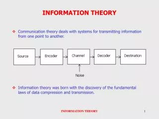
2. Encoding English in ASCII • Pop Quiz: How many bits are needed for the ASCII encoding of ”HELLO WORLD”? 11 * 8 = 88 bits

3. A Better Encoding • Suppose we assume our alphabet to be 26 letters + a space. Now what is the optimal encoding? log 27 = 5 bits per character 11 * 5 = 55 bits Can we do better than this?

4. Impossible! We know that n different possibilities can’t be represented in less than log n bits. So log n is optimal.

5. Be careful what you mean by “optimal”! log n is optimal only for a certain (very simple) model of English. By using more sophisticated models, we can achieve better compression! Oh.

6. English Letter Frequencies • In English, different letters occur with different frequencies. ETAONIHSRDLUMWCFGYPBVKQXJZ

7. Morse Code • Morse Code takes advantage of this by assigning shorter codes to more frequently occurring words:

8. Morse Code • Let’s encode our original message in Morse Code, using 0 for dot and 1 for dash: 00000010001001110111110100100100 (32 bits) When this is received at the other end, it is decoded as: IIFFETG MTGXID What went wrong?

9. What Went Wrong • Morse Code actually uses four symbols, not two. In addition to the dot and dash, we have a letter space and a word space: • .... . .-.. .-.. --- / .-- --- .-. .-.. -.. • Computers only have two symbols. How can we separate our characters?

10. A Code As a Binary Tree 0 1 A = 00 B = 010 C = 1 D = 011 E = 0 F = 11 E C 0 0 1 1 A F 1 0 D B

11. Prefix-Free Codes A = 100 B = 010 C = 101 D = 011 E = 00 F = 11 0 1 0 1 0 1 E F 1 1 0 0 A C D B

12. What kinds of codes can be prefix-free?

13. Kraft Inequality • There is a simple necessary and sufficient condition on the lengths of the codewords: • A prefix-free code with lengths {l1, l2, …, ln} satisfies the inequality: Conversely, given any set of lengths satisfying this inequality, there is a prefix-free code with those lengths.

14. lmax levels leaves beneath a node Proof of the Kraft Inequality D F E B A C

15. Proof of the Kraft Inequality

16. l2 l1 l3 l5 l4 l6 l7 Converse to the Kraft Inequality • Given a set of lengths {l1, l2, …, ln}, where l1 l2  …  ln :

17. Prefix-Free Code for English • If we restrict ourselves to prefix-free codes, we get a more modest code for English:

18. What Is an Optimal Code? • Now that our codewords don’t all have the same length, we need a slightly more sophisticated notion of “optimal”: • OLD DEFINITION: shortest codeword length NEW DEFINITION: shortest weighted average codeword length

19. Aside: Expected Values • If we have a probability distribution X on real numbers such that xi occurs with probability pi, then the expected valueE[X] of this distribution is the weighted average of the values it can take on:

20. Given an alphabet and a set of frequencies, what is the optimal code?

21. Claude Shannon (1916-2001) “The Father of Information Theory”

22. Shannon Source Coding Theorem • Given an alphabet A and a prefix-free code for A: • Let pi be the probability of character ai • Let li be the length of the codeword for ai • Then:

23. (x2, log x2) (E[x], log E[x]) (x1, log x1) (E[x], E[log x]) E[x] x1 x2 Lemma: log E[X]  E[log X]

24. (E[x], log E[x]) (E[x], E[log x]) E[x] Lemma: log E[X]  E[log X] x4 x2 x3 x1 x5

25. Proof of the Source Coding Theorem

26. Notice that we have found a lower bound on the compression possible independent of the type of objects we are encoding or their original representation! All that matters is the number of different possibilities and their distribution.

27. This quantity H = E[log 1/p] can be seen as the average amount of information contained in a message. The source coding theorem says that you cannot represent a message using fewer bits than are truly in the message.

28. H(X) is called the entropy of a probability distribution X

29. Entropy of a Biased Coin

30. The entropy can also be seen as the amount of uncertainty in a probability distribution.

31. Getting Close to the Entropy • The source coding theorem says that the entropy is a lower bound on our compression. However, we can easily achieve compression within one bit of the entropy. Thus, if L* is the expected length of the optimal code for distribution X:

32. Shannon-Fano Coding • For each letter appearing with probability p, assign it a codeword of length log 1/p. • These lengths satisfy the Kraft inequality: Therefore, there is a prefix-free code with these lengths. Since we are less than one bit away from optimal on each code word, we have:

33. The Story So Far… • We have shown that the entropy is a lower bound on compression, and we can achieve compression with one bit of the entropy: Can we do better than H(X) + 1?

34. Getting Closer to the Entropy • Instead of encoding single characters, we encode blocks of length n. Xn is the distribution on these blocks, such that p(x1x2…xn) = p(x1) p(x2) … p(xn).

35. Consider a biased coin with p = .99, q = .01 The Shannon-Fano code assigns lp = 1 and lq = 6 p q Shannon-Fano is Not Optimal • Even though we can get arbitrarily close to the entropy, Shannon-Fano coding is not optimal. Huffman coding creates a pruned tree and an optimal code.

36. An Optimal Code for English • Here is a Huffman code based on the English letter frequencies given earlier: H = 4.16, L = 4.19. Can we do better?

37. Hmm… we should be careful. Huffman coding is optimal for a simple model that only looks at letter frequencies. Maybe we can do better! You’re actually learning something, Bonzo.

38. English Digrams • Some two-letter combinations are much more likely than others. For instance, U is the most likely letter to follow Q, even though U is not the most frequent overall. How can we take advantage of this structure?

39. and: Taking Advantage of Digrams • We can take advantage of the digram structure of English by having 27 different codes, one for each letter + space. If the probability that letter j follows letter i is pi(j), then we have:

40. Similarly, we could exploit the trigram structure of English (using 272 codes), or we could encode whole words at a time. The more structure we include in our model of English, the lower the entropy and the better we can compress.

41. There are varying estimates to the True Entropy of English, but they are around 1 bit per character! Wow!

42. Each new letter gives very little information—it is mostly repeating structure we already knew. In other words, English is highly redundant. Our goal in compression is to eliminate redundancy.

43. You are much more likely to get this email: Hey, let’s go to lunch. 12:30 tomorrow? than this one: lk sl kja4wu a dl se46kd so356? lsafd! Redundancy in English • Stated more precisely, English is redundant because not all messages of the same length are equally probable.

44. Compression is a redistribution on bitstrings so that all strings of length k have probability about 2-k—giving the maximum entropy possible in k bits.

45. What if we have noise on our channel? You have toys in your flannel??

46. Noisy Communication • A noisy channel will randomly distort messages. You could send: Meet me in the park--Gary. and it could be received as: Beat me in the dark, baby! Clearly, this poses problems. We need a code that allows for error detection, or better, correction.

47. An Error Correcting Code • The “phonetic alphabet” used by aviators and the military is an error-correcting code for speech:

48. How do we do error correction on a binary channel?

49. Binary ECCs/EDCs • Method 1: Repeat bits Send each bit n times instead of just once. On the receiving end, take the majority of each n-bit block. 0110101  0000 1111 1111 0000 1111 0000 1111 (n = 4) Pros: Corrects up to (n-1)/2 errors per block Cons: Message expands by a factor of n; rate goes to 0 as n 

50. Binary ECCs/EDCs Method 2: Use a parity bit • After every n-bit block, send the parity of the block. On the receiving end, check the parity for consistency. • 01100101  011001010, 10011011  100110111 • Pros: Detects an odd number of bit flips with only 1/n extra bits • Cons: Cannot detect an even number of flips, cannot correct errors