Optimizing Experimental Data Analysis: Inference, Hypothesis Testing, and Error Control
Understand inferential statistics, hypothesis testing, and error variances in data analysis. Learn to analyze group differences, correct errors, and boost research reliability.

Optimizing Experimental Data Analysis: Inference, Hypothesis Testing, and Error Control
E N D
Presentation Transcript
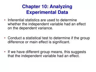
Chapter 10: Analyzing Experimental Data • Inferential statistics are used to determine whether the independent variable had an effect on the dependent variance. • Conduct a statistical test to determine if the group difference or main effect is significant. • If we have different group means, this suggests that the independent variable had an effect.
BUT, there can be differences between the group means even if the independent variable does not have an effect • The means will almost never be exactly the same in different conditions • Error variance (random variation) in the data will likely cause the means to differ slightly • So the difference between the two groups must be bigger than we would expect based on error variance alone to conclude it is significant. • We use inferential statistics to estimate how much the means would differ due to error variance and then test to see whether the difference between the two means is larger than expected based on error variance.
Hypothesis testing • Null Hypothesis (H0): states that the independent variable did not have an effect. • The data do not differ from what we would expect on the basis of chance or error variance • Experimental Hypothesis (H1): states that the independent variable did have an effect. • If the researcher concludes that the independent variable did have an effect they reject the null hypothesis. • groups means differed more than expected based on error variance
If they conclude that the independent variable did not have an effect they fail to reject the null hypothesis • Groups means did not differ more than expected based on error variance. Type I error: when you reject the null hypothesis when is in fact true. • The researchers conclude that the independent variable had an effect, when in reality it did not have an effect. • The probability of making a type 1 error is equal to alpha ().
Most researchers set = .05 meaning that they will make a type I error not more than 5 times out of 100. • There is a 95% probability they will correctly conclude there is a difference and a 5% probability they will conclude there is a difference when there was not a real difference. • If you set = .01 ( more conservative). You know that only 1 out of 100 times would expect to find a difference when there really is no difference. • 99% confident your results are do to a real difference and not chance or error variance.
Type II error: fail to reject the null hypothesis when the null hypothesis is really false. • The researcher concludes that the independent variable did not have an effect when it fact it did have an effect. • The probability of making a type II error is equal to beta (). • Many factors can result in a type II error: unreliable measures, mistakes in data collecting, coding, and analyzing, a small sample size, very high error variance.
Power of a test is the probability that the researchers will be able to reject the null hypothesis if the null hypothesis is false. • The ability of the researchers to detect a difference if there is a difference • Power = 1 - • Type II errors are more common when the power is low.
Power is related to the number of participants in a study, the greater the number of participants the higher the power. • Researchers may conduct a power analysis: to determine the number of participants they would need to detect a difference. • Power of .80 higher is considered good (80% chance of detecting an effect if there is an effect). • If the power is .80 then beta is .20. • Alpha is usually set at .05, but beta at .20, because it is worse to make a Type I error (saying there is a difference when there really is not) than a type II error (fail to find a difference when there really is a difference)
Effect Size: index of the strength of the relation between the independent variable and the dependent variable. • The proportion of variability in the dependent variable that is due to the independent variable • ranges from .00 to 1.00 • If the effect size is .39, this means that 39% of the variability in the dependent variable is due to the independent variable.
T test: • An inferential test used to compare to means Step 1: calculate the mean of the two groups Step 2: calculate the standard error of the difference between the two means • how much the means are expected to differ based on error variance • 2a: calculate the variance of each group • 2b: calculate the pooled standard deviation Step 3: Calculate t Step 4: Find the critical value of t Step 5: Compare calculated t to critical t to determine whether you should reject the null hypothesis.
Paired t-test: is used when you have a within subjects design or matched subjects design. The participants in the the condition are either the same (within) or very similar (matched). • This test takes into account the similarity in the participants • More powerful test because the pooled variance is smaller resulting in a larger t. • Computer analyses: are now used to conduct most tests.
Chapter 10: Analyzing Complex Designs • T-tests are used when you are comparing two means. But what if there are more than two levels of the independent variable or two-way design? • You could do separate t tests on all the means. But the more tests you conduct the increased chance of making a type I error. • If you made 100 comparisons, you would expect 5 to be significant by chance alone (even if there is no effect). • If you did 20 tests you would expect about 1 to be significant by chance (Type I error).
Bonferroni adjustment: used to adjust for the Type I error rate. • Divide the alpha level (.05) by the number of tests you conduct. • If doing 10 tests: (.05/10 = .005). Which means you must find a larger t for it to be significant (more conservative). • But this also increases your chance of making a Type II error (missing an effect when there really is one).
Analysis of Variance (ANOVA) • Used when comparing more than two means in a single factor study (one-way) or in a study with more than one factor (two- and three-way etc.). • Analyzes differences between means simultaneously, so Type I errors are not a problem. • Calculates the variance within each condition (error variance) and the variance between each condition. • If we have an effect of the independent variable then there should be more variance between conditions than within conditions.
F-test: divide the between groups variance by the within groups variance. If larger the effect of the independent variable the larger the F 11 10 9 8 8 7.5 7 6 5.5 5 4 3 2 1 1
Total Sums of Squares • Subtract the mean from each score, square the difference, and then add them up. • SStotal is the total amount of variability in all the data. Sum of Squares within Groups • SStotal Sum of Squares b/w Groups
Sum of Squares Within-Groups (SSwg) • calculate the sum of the squares for each condition and then add these together. • This is the variability that is not due to the independent variance (error variance) • To get the average SSwg you must divide SSwg by the degrees of freedom (dfwg). • df is represented by n - k, n = sample size and k = number of groups or conditions. • SSwg/ n- k = MSwg (mean square within-groups)
Sum of Squares Between Groups: SSbg • calculate the grand mean (mean across all conditions). • If there is no effect of the IV all condition means should be close to the grand mean. • Subtract the grand mean from each of the condition means, squares these differences, and multiply this by the size of the group, and then sum across groups. • To get an average of the SSbg you must SSbg/ dfbg • df: k - 1 (number of groups minus 1) • SSbg / dfbg = MSbg (mean square between-groups)
This reflects the differences among the groups that is due to the independent variable, but there still may be some differences that are due to error variance (random variation).
F-test • Test whether the mean variance between groups is larger than the mean variance within groups. • F = MSbg/ MSwg • If there is no effect of the independent variable the F value will be 1 or close to 1, the larger the effect the larger the F value. • Compare your F value to the critical F value using tables in text. • Need the alpha level (.05) and dfbg and dfwg • If your F is larger than the critical F then you can conclude that your independent variable had an effect or there is a significant main effect
Factorial Design • More than one independent variable (two-way) Calculate the Mean Square (MS) for the error variance (within groups), independent variable A and B, and the interaction between A and B. • FA = MSA/MSwg • FB = MSB/MSwg • FAxB = MSAxB/MSwg
B 1 2 1 2 A
Follow-Up Tests • If you have more than two levels of the independent variable the ANOVA will tell you if there is an effect of the independent variable, but it will not tell you which means differ from each other
A B C
Can do follow-up tests (post hocs or multiple comparisons) to test for differences among the means. Can test mean A against B and C, and B against C. • It could be that all three means differ from each other, or it could be that only B and C differ but A does not differ from B. • You ONLY conduct follow-up tests if the F-test was significant.
Interactions • If the interaction is significant we know that the effect of one independent variable differs depending on the level of the other independent variable. • In a 2 x 2 design (independent variable A and B) • Simple main effect: the effect of one independent variable at a particular level of another independent variable • Simple main effect of A at B1, A at B2, B at A1, B at A2.
B 1 2 1 2
B 1 2 1 2 3 A
Multivariate Analysis of Variance (MANOVA) • Used when you have more than one dependent variable. • Test differences between two or more independent variables on two or more dependent variables • Why not just conduct separate ANOVAs? • MANOVA is usually used when the researcher has dependent variables that may be conceptually related • Control the Type I error rate (tests all dependant variables simultaneously)
MANOVA creates a new variable called the canonical variable (a composite variable that is a weighted sum of the dependent variables). • First, test to see if this is significant (multivariate F) and then conduct separate ANOVAs on each dependent variable.