Download
1 / 37
370 likes | 548 Vues
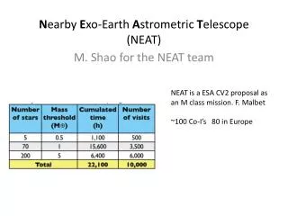
N earby E xo -Earth A strometric T elescope (NEAT). NEAT is a ESA CV2 proposal as an M class mission. F. Malbet ~100 Co-I’s 80 in Europe. M. Shao for the NEAT team. Intro. Towards discovery and characterization of Exo -Earths Eta_earth from RV (Astrometry and Direct Detection)

E N D
Nearby Exo-Earth AstrometricTelescope (NEAT) NEAT is a ESA CV2 proposal as an M class mission. F. Malbet ~100 Co-I’s 80 in Europe M. Shao for the NEAT team
Intro • Towards discovery and characterization of Exo-Earths • Eta_earth from RV (Astrometry and Direct Detection) • In astrometry with a telescope, what are the major obstacles, that led us to the SIM design? • HST, Kepler, etc? • Photon noise. WFPC3 has a ~3 arcmin field. Brightness of ref stars ~ area of FOV. (SIM’s 2 deg DIA, ~2000 bigger) • Beam walk (optical errors). The stellar footprint on secondary, tertiary is different for different stars in the FOV. • Focal plane array stability. (Mosiac of ccd’s) • Intra-pixel QE variations/PSF. (even in a narrow field, the stars move ~0.2 arcsec due to diff stellar abberation, also PM, parallax)
Is AstrometricExo-Earth Discovery Scientifically Important? • Can RV find nearby Earths? • A. Howard gave a good review of our current understanding. • A lot of work has been done and continues on what is the ultimate limit in RV due to astrophysical noise. • G. Marcy ,S. Udry, and D. Queloz, are all on the NEAT science team. • Ignoring meridonal flows, under the most optimistic assumptions (brightest ~dozen) Expresso might get to 2 Mearth. (lots of telescope time) • The Expresso target list will consist of the (RV)quietest ~50 targets, at a mean distance of ~40 parsec. (as of mid 2009) The vast majority of these targets can’t be followed up by a 4m or even 8m coronagraph. (25?mas R_max)
The distribution of HOT Terrestrial mass planets was estimated by the Berkeley Eta_earth survey of nearby FGK stars. The estimates are based on detected planets, candidate planets as well as an estimate of the “missed” planets. For HOT Earths P < 50 days 1-3 Mearth ~14% (+8%, -5%) 3-10 Mearth 12% (+4.3%, -3.5%) Howard et. al. Science Vol 330 P653, Oct 2010 http://www.sciencemag.org/content/330/6004/653.full.pdf if we assume uniform density in log P, (log (50/2) / log(1.6yr/0.6yr))~3 Hab Zone Planets 1-3 Me 4.7% Hab Zone Planets 3-10 Me 4.0% A search of 35 stars will have a 95% chance of finding 1 or more 1-10 Me planets in the HZ. (on average find 3 planets) A search of 64 stars will have a 95% chance of finding 1 or more 1-3 Me planets in the HZ. (on average find 3 planets)
The unique capability of a direct detection mission is to measure the spectra of the planet, in the visible to find oxygen in the atmosphere. The table below gives the size of the telescope needed to detect oxygen in an exo-earth around the nearest N stars. 95% chance of finding and characterizing at least 1exo-Earth (in HZ) Separating planet from exo-zodi is much easier At 4 l/D than at 2 l/D.
NEAT is a ESA CV2 proposal as an M class (~450M Euro )mission. 1m telescope and focal plane with < 3Mpix
Major Technical Issues for uas Astrometry • In astrometry with a telescope, what are the major obstacles, that led us to the SIM design? • Photon noise. The target stars are bright, photon limit is from the reference stars (SIM’s 2 deg DIA) • Beam walk (optical errors). The stellar footprint on secondary, tertiary is different for different stars in the FOV. (more on this later) • Focal plane array stability. (Mosiac of ccd’s) (1e-11) • Intra-pixel QE variations/PSF • Pixels are not uniformly spaced @ 1e-5 pixels • Pixel QE’s are not uniform across 1 pixel to 1e-5 • The Optical PSF changes by lambda/100 across the field. • Centroiding to a few*1e-3 pixels has been demonstrated. • SIM related technology provides solutions to the last 2 problems
Photon Noise • Nominal 1m telescope 0.36 sqdegfov • 0.71 uas in 1 hr (photon limit from ref stars) • SIM-Lite performance 1.0 uas 2axis, in 1 hr R band 640nm 25% bw Total QE 60% (ideal 85%) Use photons from brightest 6 ref stars # ref stars (avg for sky from AQ4) #ref stars 5 6 7 10 100 phot noise 0.73 0.71 0.69 0.65 0.52 uas faintest 11 11 11 12 14 mag CCD can run at 25C (but very slightly better at 0C) If target star < 8 mag, photon noise from target not important Photon noise from laser metrology not important. Lasers turned on ~3% of time, every ~ minute (depending on therm stab)
Beam Walk Error in Normal Telescope • 1 uas (across a 1m mirror) is 5 picometer/1m. 1/20 the diameter of an atom. • If the secondary surface is not perfect • at the 5pm level there will be systematic biases > 1uas. • Biases that are constant (for 5yrs) are OK. But 5pm stability is not possible for any optic over 5 yrs. Detailed simulation results of Beam walk error in a 3 mirror TMA telescope (O. Guyon) would be 0.5~1 milliarcsec if the secondary and tertiary optics are polished to 1nm accuracy. Beam walk errors are smaller for smaller angles ~10uas for 10 arcsec field.
NEAT Telescope Concept Fibers attached To ULE primary Produces fringes At focal plane Concept: 1m OAP, 40m focal length, 2 spacecraft fly in formation (L2), or deployed boom (backup) focal plane of 9 (256*256?) CCDs 8 on X,Y stages. Laser system for focal plane metrology Beamwalk: There’s only 1 optic, no beam walk Fibers attached to ULE/Zerodur primary monitors focal plane geometry. Intra-pixel QE/PSF model each pixel modeled with <QE>, and 5 other parameters that specify QE(x,y) within a pixel. Centroid PSF to 10-5 pix Photon noise. Brightest 8 stars in a 0.6*0.6 deg box. Cost of giga pixel focal plane, replaced by cost of 9 256*256 CCDs and 8 x,y stages
Telescope – Deployed Version Primary Mirror Focal Plane View from Top Looking Down Focal Plane location Light baffle Primary Mirror location Fully Deployed Spacecraft
Focal Plane Concept 8 Movable CCDs 0.1 uas across 0.6deg is 4x10-11. A mosiac of CCD’s made of many materials with different CTE, will not be stable to 4x10-11for 5 yrs. even 10-5 pix over 4000pix within 1 CCD is 2x10⁻⁹ difficult The CCDs for the ref stars move. Put the star on the same set of pixel(s) at every epoch Position of CCD monitored by laser metrology across the full FOV 10-5 pix over 32*32pix is 3x10⁻⁷ requires < ~0.1K long term (Si) fixed 0.6 deg We measure the PSF centroid with respect to the laser fringes, using the CCD pixels as an intermediary.
Pointing Stability • The target star is very bright, 32*32 pix area read out at 1Khz. • The centroid (in real time) is fed to a momentum compensated (primary) tip/tilt mechanism to keep the image on the focal plane stable at ~0.5 mas. • The spacecraft(s) pointing should be a fraction of an arcsec. • Our current operations concept is to turn on the metrology for ~1 sec every 10sec to 1 minute, during a typical 2 hr observation of a target. We measure the position of a group of ~32*32 pixels over time. • When analyzing metrology data, the stellar light is treated as “background”. A group of 32*32 pixels (300*300um) should be stable to 10-5 pix if the CCD temperature is stable to 0.1K. Momentum comp tip/tilt stage on telescope primary Target star ccd 1Khz Closed loop pointing
Calibrating CCD Centroiding Errors • Two classes of errors • Pixels move. Measure location of a group of pixels • PSF centroiding with imperfect pixels • QE(x,y,I,j) Intrapixel QE spatial variations for each pixel. • Deriving Optical PSF shape • Simulations of PSF centroiding, assumptions, and how detailed do we have to know the PSF and the QE(x,y) to centroid to ~5e-6 pixels, and how do we make the calibration measurements? • Initial CCD centroiding results.
Focal Plane: Pixel Location Calibration • Issues: • Focal plane geometry: 1 uas/0.6deg is 4e-10. A mosaic of CCDs cannot be kept this stable, CCD pixels will change geometry and move relative to each other. • Intra-pixel QE variation: Every pixel has a different geometry and QE non-uniformity between and within pixels. • Solution: • We use a “focal plane” metrology system derived from SIM heterodyne metrology to precisely monitor the CCD relative locations and to calibrate each pixel (geometric position, QE(I,j) response and QE non-uniformity QE(x,y)). Focal plane fo Primary mirror Optical fibers Fringe motion D fo+5Hz F
MicropixelCentroidTesbed • 10-5 pixel centroid measurements are needed for 1uas astrometry. Current state of the art is about ~2x10-3 pixel. • The graph shows the spatial fringes across 80pixels. • The fringes move (left to right) at ~5hz, images are recorded at 50hz. • If the fringe motion is uniform, then one pixel’s output is C0+C1*sin(w*t + phi(I,j)) • Phi(i,j) gives us the location of the pixel fo+5Hz Fringe motion fo Fibers mounted to edge of Zerodur parabola CCD
Testbed Results: Measuring Pixel Motion • If we were to fit a static fringe pattern across many pixels, the QE variations that are unknown would bias the pixel position. • Instead, with heterodyne fringes, we measure the position of a pixel by looking at that pixel’s flux versus time (phase of a sine wave in time). • We have demonstrated 2 10-5 pixel position measurement error for groups of 10x10 pixels in less than 25 seconds of integration. 10x10 pixel areas < 1 10-4 pixel in 1s < 2 10-5 pixel in 25s
Testbed: Next Step • Conduct 2D (X,Y) measurements of pixel position. • Put pseudo-star images on the CCD and demonstrate centroiding to 10-5 pixels. Metrology fibers fo+1Hz Starlight fiber bundle at the focus of the parabola CCD Pseudo-star images fo Focal-plane metrology
Star Centroiding to 10-5 pixel Point Spread Function (PSF) definitions: • True PSF: Image(x,y) at infinite spatial resolution. • Model PSF: Our guess of what the true PSF is. • Pixelated PSF: I(i,j), the integral of Image(x,y)·QEi,j(x,y)·dx·dy Classical Approach for centroiding: • Perform Least-Square Fit of CCD data to the pixelated model PSF, fitting for x, y, intensity. • Known problems: • True PSF differs from model PSF, true PSF changes with star color, position in FOV, and as the optics warp. But more important, the model PSF is not the true PSF. • Calculating the pixelated PSF from the model PSF requires knowledge of QE(x,y) within every pixel. • The canonical approach to measuring QE(x,y) is to scan a spot across each pixel. No done because of practical reasons: can’t do all pixels at once, diffraction pattern spills over to next pixel, knowledge of the scanning spot position. NEAT Approach for centroiding: • Nyquist theorem: Critically sampling a band limited function at greater than 2*bandwidth is sufficient to perfectly reproduce that function. • We have the knowledge of the true PSF in the data, not a guess of the true PSF. • We use laser metrology to measure QE(x,y) for all pixels simultaneously. In fact, we measure the Fourier Transform of QE(x,y), by putting fringes of various spacing and directions across the CCD. • Numerical simulations show that QE(x,y) calibrated with 6 parameters per pixel is sufficient for ~2x10-6 pixel centroiding for a backside CCD with P-V QE variation <10% across pixel.
Measure pixel position and QE(x,y) within each pixel. By putting fringe patterns across the CCD with different fringe spacing and orientation. QE MTF is measures the fourier transform of QE(x,y) is measured. • Numerical simulations show that QE(x,y) calibrated with 6 parameters per pixel is sufficient for ~2x10-6 pixel centroiding for a backside CCD with P-V QE variation <10% across pixel (assuming intra-pixel QE varies by <6%).
Images are Nyquist Sampled> 2 pixel /(l/D) True optical PSF derived from pixelated PSF. 3 stellar images on CCD
Centroid Allan Deviations Single Fiber centroid reaches noise floor at 3e-4pixels (drift) Differential centroid continue to average down to ~4e-5 pixels after 100 sec integration A C B
Calibrating vs Averaging CCD Errors • Without sub-pixel calibration, CCD pixelation and imperfect PSF models will produce a few~3*10-3 pixel errors. • One can calibrate sub-pixel QE variations, with very high accuracy to get 1e-6 pixel centroiding. OR • One can move the image to 107 different statistically independent positions on the CCD and average down the hopefully random errors down to 10-6 pixels. • Or one can use a combination of the two approaches. • The question of asking sqrt(N) to provide accuracy gives rise to the question, are the errors really random at that level? If one is measuring the distance between 2 stars as the two stars are moved across many CCD pixels, might have systematic errors if the spacing between pixels slowly varies across the chip. • The use of laser metrology to define the CCD pixel geometry can go a long ways to removing the type of systematic error that prevents averaging to large N • The approach we’ll most likely use in NEAT is to calibrate close the the requirement, then use sqrt(N) for the last factor of a few. • Ref stars ccd’s will be read out at ~50 hz, in 2 hrs we’ll have 360K images.
A Possible Addition to NEAT(Not supported by the NEAT science team) • We made a case that astrometry can, needs to and should find the exo-Earths around ~75 nearby stars. • A direct detection mission that can search 75 stars and get spectra @800nm needs a large telescope (5~10m) • We also need to know the level of exo-zodi around stars with exo-Earths, if we want to be able to specify the size of the coronagraph to 20% instead of +/- 5 Billion$. A 10m telescope may be needed because all stars have high (3~10) exo-zodi levels. • The NEAT telescope is compatible with all existing coronagraph concepts. The 1m aperture is a bit small, but measuring exo-zodi at 500nm (not 800nm) and at 1.5~2AU will give us a good idea of the exo-zodi environment, of the stars that have exo-Earths. This provides a solid foundation for a direct/spectroscopic mission.
Request to the EXOPAG • Endose NEAT , finding nearby earths should be a high priority of any explanet program. • Communicate this to NASA and to ESA • Endorse NASA participation in NEAT • EXOPAG Consider/analyse NASA adding to NEAT a high performance coronagraph to study exo-zodi of nearby stars. • The best way, perhaps the only way to reduce the “perceived cost” of a space coronagraph is to fly a coronagraph in space. (At the cost of an instrument, not the cost of a mission, in an environment where failure to achieve 1e-10 contrast doesn’t result in total mission failure. Making science measurements (exo-zodi) that is scientifically dull, but absolutely necessary for any future direct detection mission.)
Ground Detection of Jupiters, Reflected Light Sun-Jupiter @ 5AU has a contrast of 1e-9 At 0.5AU the contrast is 1e-7. At 10pc this is 50 mas. 1.2um/30m = 8.3mas. Jupiter is at 6 l/D On the ELT 42m this is 8.4 l/D (The baseline coronagraph for TMT is a vis Nulling coronagraph. But also the segmented aperture is less serious at 1e-7 rather than 1e-10 contrast.)
IWA = 2 l/D Planet @ 2 l/D Exozodi=1 => Exozodi ~12X planet IWA = 4 l/D Planet @ 4.5 l/D Exozodi=1 => Exozodi ~3X planet Exo-zodi surface brightness is constant, higher angular resolution means exozodi flux per airy spot is smaller.
Control of Focal Plane Errors • Two types of focal plane errors • Pixel location. (accracy of pixel placement not important, stability over 5 years is) (0.3~1.0x10-5 pixels) • PIAA concept solves this problem by only doing astrometry within 1 CCD. (20 arcsec local astrometry ref star and nearby diff spike on the same chip, 0.2uas/20uas ~ 10-8 does this sqrt(N) down?) • In our concept we measure the position of the chip with a laser system. (no photon penalty of faint diff spikes) • CCD QE errors (QE(x,y) and its effect on PSF centroiding) uncalibrated, this error is 0.01~0.03 pixels. • PIAA concept solves this by sqrt(N). Here N~ 106 from 0.01pix to 10-5 pix. Rotation around LOS ~90deg. • Our concept, calibration of Pixel location and QE(x,y) along with repeatedly putting the star on the same part of the same pixel at every epoch.
Stability of Focal Plane Fringes • The fringes produced by the fibers near the primary are used to measure the distance between every pixel in the focal plane. How stable do the fringes have to be? • The fringes are used the measure the distance between pixels. The fringes sweep by at ~5hz. The “phase” of the fringe at pixel “a” is compared to the phase at pixel “b”. The distance between pixels is measured in units of fringes. (l/a, a is the angle between interfering beams) The wavelength of the laser will be very stable but what about a? ~100 years ago astrometrists used the affine transformation to correct for “simple” geometric errors in the focal plane by using the position of “reference” stars to solve for the “Plate” parameters ABCDEF. That represent X,Y origin, X,Y scale, rotation of the image and rotation of the X vs Y axis. Using this approach there is no requirement for stability of the fibers location. Xt = A*Xm + B*Ym + C Yt = D*Xm + E*Ym + F
Cost Implications • The great reliance on sqrt(N) to average out errors => a fully populate focal plane ~ 109 pixels. The Kepler 108 pix focal plane is ~$38M. • Rotation implies a very large data volume. If an image is recorded for every 1/10 pixel rotation of the FOV, the data volume is ~50 Terabytes per observation (2 days). • 20 arcsec around 1000 ref stars is ½ the focal plane. Reduction in the data volume by 100~1000X is needed to fit within the capabilities of the DSN. (worst case) • Best case still being investigated • The long focus telescope design needs a long deployed boom. (some way to hold the focal plane a long distance from the primary)
Dynamic (vs static) Focal Plane Metrology • With static focal plane metrology the fringes are stationary. We centroid the fringes vs the stars. • With static fringes, all the intra pixel QE errors affect the centroiding of the stars also affect centroiding of the fringes. • Dynamic fringes (constantly moving) does not let us measure the position of a pixel, only the distance between 2 pixels. • CCD_flux(time) = 1+ vis*sin( w*t +phi) (independent of QE variations within a pixel, as long as the QE(x,y) variations are constant in time. • Our SIM laser heterodyne metrology also uses temporal fringe modulation. • Temporal fringes from each pixel tells us (relative location to another pixel” and the pixel’s width) Fringes with periods < pixel width explore QE inside a pixel.
3D focal plane measurements 2 fibers are needed to measure motion of CCD in X 3rd fiber is needed to measure X,Y motion 4th fiber is sufficient to measure XYZ motion of the CCD. Bisector Everywhere along Bisector OPD from two fibers are equal