Lecture 18: Approximate Pattern Matching
Lecture 18: Approximate Pattern Matching. Study Chapter 9.6 – 9.8. Approximate vs. Exact Pattern Matching. Previously we have discussed exact pattern matching algorithms Usually, because of mutations, it makes much more biological sense to find approximate pattern matches

Lecture 18: Approximate Pattern Matching
E N D
Presentation Transcript
Lecture 18:Approximate Pattern Matching Study Chapter 9.6 – 9.8 COMP 555 Bioalgorithms (Fall 2012)
Approximate vs. Exact Pattern Matching • Previously we have discussed exact pattern matching algorithms • Usually, because of mutations, it makes much more biological sense to find approximate pattern matches • Biologists often usefast heuristic approaches (rather than local alignment) to find approximate matches COMP 555 Bioalgorithms (Fall 2012)
Heuristic Similarity Searches • Genomes are huge: Smith-Waterman quadratic alignment algorithms are too slow • Good alignments of two sequences usually have short identical or highly similar subsequences • Many heuristic methods (i.e., BLAST, FASTA) are based on the idea of filtration • Find short exact matches, and use them as seeds for potential match extension • “Filter” out positions with no extendable matches COMP 555 Bioalgorithms (Fall 2012)
Dot Matrix • A dot matrix or dot plot show similarities between two sequences • FASTA makes an implicit dot matrix from short exact matches, and tries to find long diagonals (allowing for some mismatches) • Nucleotide matches l = 1 COMP 555 Bioalgorithms (Fall 2012)
Dot Matrix • A dot matrix or dot plot show similarities between two sequences • FASTA makes an implicit dot matrix from short exact matches, and tries to find long diagonals (allowing for some mismatches) • Dinucleotide matches l = 2 COMP 555 Bioalgorithms (Fall 2012)
Dot Matrix • Identify diagonals above a threshold length • Diagonals in the dot matrix indicate exact substring matching l = 2 COMP 555 Bioalgorithms (Fall 2012)
Diagonals in Dot Matrices • Extend diagonals and try to link them together, allowing for minimal mismatches/indels • Linking diagonals reveals approximate matches over longer substrings l = 2 COMP 555 Bioalgorithms (Fall 2012)
Approximate Pattern Matching (APM) • Goal: Find all approximate occurrences of a pattern in a text • Input: • pattern p = p1…pn • text t = t1…tm • the maximum number of mismatches k • Output: All positions 1 <i< (m – n +1) such that ti…ti+n-1 and p1…pn have at most k mismatches • i.e., Hamming distance between ti…ti+n-1 and p <k COMP 555 Bioalgorithms (Fall 2012)
APM: A Brute-Force Algorithm ApproximatePatternMatching(p, t, k) • n length of pattern p • m length of text t • fori 1 to m – n + 1 • dist 0 • forj 1 to n • ifti+j-1 != pj • dist dist + 1 • ifdist<k • outputi COMP 555 Bioalgorithms (Fall 2012)
APM: Running Time • That algorithm runs in O(nm). • Extend “Approximate Pattern Matching” to a more general “Query Matching Problem”: • Match n-length substring of the query (not the full pattern) to a substring in a text with at most k mismatches • Motivation: we may seek similarities to some gene, but not know which parts of the gene to consider COMP 555 Bioalgorithms (Fall 2012)
Query Matching Problem • Goal: Find all substrings of the query that approximately match the text • Input: Query q = q1…qw, text t = t1…tm, n (length of matching substrings n ≤ w ≤ m), k (maximum number of mismatches) • Output: All pairs of positions (i, j) such that the n-letter substring of q starting at iapproximately matches the n-letter substring of t starting at j, with at most k mismatches COMP 555 Bioalgorithms (Fall 2012)
Approximate Pattern Matching vs Query Matching COMP 555 Bioalgorithms (Fall 2012)
Query Matching: Main Idea • Approximately matching strings share some perfectly matching substrings. • Instead of searching for approximately matching strings (difficult) search for perfectly matching substrings first (easy). COMP 555 Bioalgorithms (Fall 2012)
Filtration in Query Matching • We want all n-matches between a query and a text with up to k mismatches • “Filter” out positions that do not match between text and query • Potential match detection: find all matches of l -tuples in query and text for some small l • Potential match verification: Verify each potential match by extending it to the left and right, until (k + 1) mismatches are found COMP 555 Bioalgorithms (Fall 2012)
Filtration: Match Detection • If x1…xn and y1…yn match with at most k << n mismatches they must share l –mers that are perfect matches, with l = n/(k + 1) • Break string of length n into k+1 parts, each of length n/(k + 1) • k mismatches can affect at most k of these k+1 parts • At least one of these k+1 parts is perfectly matched COMP 555 Bioalgorithms (Fall 2012)
Filtration: Match Detection(cont’d) • Suppose k = 3. We would then have l=n/(k+1)=n/4: • There are at most k mismatches in n, so at the very least there must be one out of the k+1 l–tuples without a mismatch 1…l l+1…2l 2l+1…3l 3l+1…n 1 2 k k+ 1 COMP 555 Bioalgorithms (Fall 2012)
Filtration: Match Verification • For each l -match we find, try to extend the match further to see if it is substantial text Extend perfect match of lengthluntil wefind an approximatematch of length nwith no more than kmismatches query COMP 555 Bioalgorithms (Fall 2012)
Filtration: Example Shorter perfectmatches required Performance decreases COMP 555 Bioalgorithms (Fall 2012)
Local alignment is too slow… • Quadratic local alignment is too slow when looking for similarities between long strings (e.g. the entire GenBank database) • Guaranteed to find the optimal local alignment • Sets the standard for sensitivity • Basic Local Alignment Search Tool • Altschul, S., Gish, W., Miller, W., Myers, E. & Lipman, D.J. Journal of Mol. Biol., 1990 • Search sequence databases for local alignments to a query COMP 555 Bioalgorithms (Fall 2012)
BLAST • Great improvement in speed, with only a modest decrease in sensitivity • Opts to minimizes search space instead of exploring entire search space between two sequences • Finds short exact matches (“seeds”), explore locally around these “hits” Search space of BLAST Search space of Local Alignment COMP 555 Bioalgorithms (Fall 2012)
Similarity • BLAST only continues it’s search as long as regions are sufficiently similar • Measuring the extent of similarity between two sequences • Based on percent sequence identity • Based on conservation COMP 555 Bioalgorithms (Fall 2012)
Percent Sequence Identity • The extent to which two nucleotide or amino acid sequences are invariant A C C T G A G – A G A C G T G – G C A G mismatch indel 70% identical COMP 555 Bioalgorithms (Fall 2012)
Conservation • Amino acid changes that preserve the physico-chemical properties of the original residue • Polar to polar • aspartate glutamate • Nonpolar to nonpolar • alanine valine • Similarly behaving residues • leucine to isoleucine • Nucleotide changes that preserve molecular shape • Transitions (A-G, C-T) are more similar than Transversions (A-C, A-T, C-G, G-T) COMP 555 Bioalgorithms (Fall 2012)
Assessing Sequence Similarity • How good of a local alignment score can be expected from chance alone • “Chance” relates to comparison of sequences that are generated randomly based upon a certain sequence model • Sequence models may take into account: • nucleotide frequency • dinucelotide frequency (e.g. C+G content in mammals) • common repeats • etc. COMP 555 Bioalgorithms (Fall 2012)
BLAST: Segment Score • BLAST uses scoring matrices (d) to improve on efficiency of match detection (we did this earlier for pairwise alignments) • Some proteins may have very different amino acid sequences, but are still similar (PAM, Blosum) • For any two l -mers x1…xl and y1…yl : • Segment pair: pair of l -mers, one from each sequence • Segment score: Sli=1d(xi, yi) COMP 555 Bioalgorithms (Fall 2012)
BLAST: Locally Maximal Segment Pairs • A segment pair is maximal if it has the best score over all segment pairs • A segment pair is locally maximal if its score can’t be improved by extending or shortening • Statistically significant locally maximal segment pairs are of biological interest • BLAST finds all locally maximal segment pairs (MSPs) with scores above some threshold • A significantly high threshold will filter out some statistically insignificant matches COMP 555 Bioalgorithms (Fall 2012)
BLAST: Statistics • Threshold: Altschul-Dembo-Karlin statistics • Identifies smallest segment score that is unlikely to happen by chance • # matches above q has mean (Poission-distributed): E(q) = Kmne-lqK is a constant, m and n are the lengths of the two compared sequences, l is a positive root of: Σx,y in A(pxpyed(x,y)) = 1 where px and py are frequencies of amino acids x and y, d is the scoring matrix, and A is the twenty letter amino acid alphabet COMP 555 Bioalgorithms (Fall 2012)
P-values • The probability of finding exactly k MSPs with a score ≥ q is given by: (E(θ)k e-E(θ))/k! • For k = 0, that chance is: e-E(θ) • Thus the probability of finding at least one MSP with a score ≥ q is: p(MSP > 0) = 1 – e-E(θ) COMP 555 Bioalgorithms (Fall 2012)
BLAST algorithm • Keyword search of all substrings of length w from the query of length n, in database of length m with score above threshold • w = 11 for DNA queries, w =3 for proteins • Local alignment extension for each found keyword • Extend result until longest match above threshold is achieved • Running time O(nm) COMP 555 Bioalgorithms (Fall 2012)
BLAST algorithm keyword Query: KRHRKVLRDNIQGITKPAIRRLARRGGVKRISGLIYEETRGVLKIFLENVIRD GVK 18 GAK 16 GIK 16 GGK 14 GLK 13 GNK 12 GRK 11 GEK 11 GDK 11 Neighborhood words neighborhood score threshold (T = 13) extension Query: 22 VLRDNIQGITKPAIRRLARRGGVKRISGLIYEETRGVLK 60 +++DN +G + IR L G+K I+ L+ E+ RG++K Sbjct: 226 IIKDNGRGFSGKQIRNLNYGIGLKVIADLV-EKHRGIIK 263 High-scoring Pair (HSP) COMP 555 Bioalgorithms (Fall 2012)
Original BLAST • Dictionary • All words of length w • Alignment • Ungapped extensions until score falls below some statistical threshold • Output • All local alignments with score > threshold COMP 555 Bioalgorithms (Fall 2012)
Original BLAST: Example • w = 4 • Exact keyword match of GGTC • Extend diagonals with mismatches until score is under some threshold (65%) • Trim to until all mismatches are interior • Output result: • GTAAGGTCC • || |||||| • GTTAGGTCC From lectures by Serafim Batzoglou (Stanford) COMP 555 Bioalgorithms (Fall 2012)
Gapped BLAST : Example • Original BLAST exact keyword search, then: • Extend with gaps around ends of exact matchuntil score < threshold • Output result: GTAAGGTCCAGT || ||||| ||| GTTAGGTC-AGT From lectures by Serafim Batzoglou (Stanford) COMP 555 Bioalgorithms (Fall 2012)
Incarnations of BLAST • blastn: Nucleotide-nucleotide • blastp: Protein-protein • blastx: Translated query vs. protein database • tblastn: Protein query vs. translated database • tblastx: Translated query vs. translated database (6 frames each) COMP 555 Bioalgorithms (Fall 2012)
Incarnations of BLAST (cont’d) • PSI-BLAST • Find members of a protein family or build a custom position-specific score matrix • Megablast: • Search longer sequences with fewer differences • WU-BLAST: (Wash U BLAST) • Optimized, added features COMP 555 Bioalgorithms (Fall 2012)
Timeline • 1970: Needleman-Wunsch global alignment algorithm • 1981: Smith-Waterman local alignment algorithm • 1985: FASTA • 1990: BLAST (basic local alignment search tool) • 2000s: BLAST has become too slow in “genome vs. genome” comparisons - new faster algorithms evolve! • Pattern Hunter • BLAT COMP 555 Bioalgorithms (Fall 2012)