Liquid Solutions
Liquid Solutions. Purpose of this lecture : To introduce the activity coefficient, a partial molar property of chemical species in non-ideal solutions. Highlights

Liquid Solutions
E N D
Presentation Transcript
Liquid Solutions • Purpose of this lecture: • To introduce the activity coefficient, a partial molar property of chemical • species in non-ideal solutions. • Highlights • The activity coefficient of a species in solution is used as a measure of the departure of this species from ideal solution behaviour. • The activity coefficient of a species in solution is defined in a similar manner as the fugacity coefficient of a species in a gas/vapour mixture • Activity coefficients are related to excess Gibbs energy • Reading assignment: Section 11.8 Lecture 14
Ideal Liquid Solutions • We have already developed a model for the chemical potential of ideal solutions. • Acknowledges the fact that molecules have finite volume and strong interactions, but assumes that these interactions are the same for all components of the mixture. • This are the same assumptions used for ideal mixtures of real gases. • The chemical potential of species i in an ideal solution is given by: • (11.75) • where Gil (T,P) represents the pure liquid Gibbs energy at T,P. • For pure liquid i • (11.31) Lecture 14
Ideal Liquid Solutions • Substituting for Gil (T,P) yields: • To estimate the chemical potential of component i in an ideal liquid solution, all we require is the composition (xi) and the pure liquid fugacity (fil ). • The fugacity of a pure liquid can be calculated using: • (11.44) • For those cases in which the ideal solution model applies, we require only pure component data to estimate the chemical potentials and total Gibbs energy of the liquid phase. Lecture 14
Non-Ideal Liquid Solutions • Relatively few liquid systems meet the criteria required by ideal solution theory. In most situations, molecular interactions are not uniform between components, resulting in mixture behaviour that deviates from the ideal case. • The approach for handling non-ideal liquid solutions is exactly the same as that adopted for non-ideal gas mixtures. We define a solution fugacity, fil as: • (11.46) • To use this approach, we require experimental data or correlations pertaining to the specific mixture of interest Lecture 14
Lewis-Randall Rule • The ideal solution model is known as the Lewis-Randall equation: • (11.83) • The solution fugacity of component i in an ideal solution (gas or liquid) can be represented by the product of the pure component fugacity and the mole fraction. • Whenever you apply an ideal solution model, you are using the Lewis-Randall rule. • This is an approximation that yields reasonable results for similar compounds (benzene/toluene, ethanol/propanol) • Is it good for ethanol and water? Lecture 14
Liquid Phase Activity Coefficients • Based on our definition of solution fugacity: • (11.46) • we could define a liquid phase solution fugacity coefficient: • that reflects deviations of the solution fugacity from a perfect gas mixture. • A more logical approach is to measure the deviations of the solution fugacity from ideal solution behaviour. For this purpose, we define the activity coefficient: • (11.90) • this convenient parameter is used to correlate non-ideal liquid solution data, just as i is used for gas mixtures Lecture 14
Excess Properties of Non-Ideal Liquid Solutions • Most of the information needed to describe non-ideal liquid solutions is published in the form of the excess Gibbs energy, GE. • Excess properties are defined as the difference between the actual property value of a solution and the ideal solution value at the same T, P, and composition. • ME(T,P, xn) = M(T,P, xn) - Mid(T,P, xn) (11.85) • What is the difference between an excess property and a residual property? • Partial excess properties can also be defined: • MiE(T,P, xn) = Mi(T,P, xn) - Miid(T,P, xn) (11.88) • where Lecture 14
Excess Properties of Non-Ideal Liquid Solutions • The partial excess Gibbs energy is of primary interest: • where • and • Leaving us with the partial excess Gibbs energy: • (11.91) Lecture 14
Excess Properties of Non-Ideal Liquid Solutions • Why do we define excess properties for liquid solutions? • They are more easily obtained from experimental data • Activity coefficients are partial molar properties with respect to excess properties. Three important results follow: • (11.96) • The Gibbs-Duhem equation: • (11.14) • The summability relation, providing GE from lni data: • (11.99) • Why is any of this important? Lecture 14