Image Alignment and RANSAC: Solving for Homographies and Robust Alignment Algorithm
550 likes | 684 Vues
This lecture covers techniques for estimating translations, affine transformations, homographies, and robust image alignment using RANSAC. Learn how to solve for homographies and align images accurately. Understand the RANSAC algorithm, its benefits, and the process of finding the best alignment through robust hypothesis generation and inlier voting.

Image Alignment and RANSAC: Solving for Homographies and Robust Alignment Algorithm
E N D
Presentation Transcript
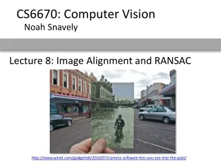
CS6670: Computer Vision Noah Snavely Lecture 8: Image Alignment and RANSAC http://www.wired.com/gadgetlab/2010/07/camera-software-lets-you-see-into-the-past/
Reading • Szeliski Chapter 6.1
Estimating Translations • Problem: more equations than unknowns • “Overdetermined” system of equations • We will find the least squares solution
Least squares formulation • For each point • we define the residuals as
Least squares formulation • Goal: minimize sum of squared residuals • “Least squares” solution • For translations, is equal to mean displacement
Least squares formulation • Can also write as a matrix equation 2n x 2 2x 1 2n x 1
Least squares • Find t that minimizes • To solve, form the normal equations
Affine transformations • How many unknowns? • How many equations per match? • How many matches do we need?
Affine transformations • Residuals: • Cost function:
Affine transformations • Matrix form 6x 1 2n x 1 2n x 6
Homographies p’ p • To unwarp (rectify) an image • solve for homography H given p and p’ • solve equations of the form: wp’ = Hp • linear in unknowns: w and coefficients of H • H is defined up to an arbitrary scale factor • how many points are necessary to solve for H?
Solving for homographies 2n × 9 2n 9 Defines a least squares problem: • Since is only defined up to scale, solve for unit vector • Solution: = eigenvector of with smallest eigenvalue • Works with 4 or more points
Image Alignment Algorithm Given images A and B • Compute image features for A and B • Match features between A and B • Compute homography between A and B using least squares on set of matches What could go wrong?
Robustness outliers
Robustness • Let’s consider a simpler example… • How can we fix this? Problem: Fit a line to these datapoints Least squares fit
Idea • Given a hypothesized line • Count the number of points that “agree” with the line • “Agree” = within a small distance of the line • I.e., the inliers to that line • For all possible lines, select the one with the largest number of inliers
Counting inliers Inliers: 3
Counting inliers Inliers: 20
How do we find the best line? • Unlike least-squares, no simple closed-form solution • Hypothesize-and-test • Try out many lines, keep the best one • Which lines?
RAndom SAmple Consensus Select one match at random, count inliers
RAndom SAmple Consensus Select another match at random, count inliers
RAndom SAmple Consensus Output the translation with the highest number of inliers
RANSAC • Idea: • All the inliers will agree with each other on the translation vector; the (hopefully small) number of outliers will (hopefully) disagree with each other • RANSAC only has guarantees if there are < 50% outliers • “All good matches are alike; every bad match is bad in its own way.” – Tolstoy via Alyosha Efros
RANSAC • Inlier threshold related to the amount of noise we expect in inliers • Often model noise as Gaussian with some standard deviation (e.g., 3 pixels) • Number of rounds related to the percentage of outliers we expect, and the probability of success we’d like to guarantee • Suppose there are 20% outliers, and we want to find the correct answer with 99% probability • How many rounds do we need?
RANSAC y translation set threshold so that, e.g., 95% of the Gaussian lies inside that radius x translation
RANSAC • Back to linear regression • How do we generate a hypothesis? y x
RANSAC • Back to linear regression • How do we generate a hypothesis? y x
RANSAC • General version: • Randomly choose s samples • Typically s = minimum sample size that lets you fit a model • Fit a model (e.g., line) to those samples • Count the number of inliers that approximately fit the model • Repeat N times • Choose the model that has the largest set of inliers
How many rounds? • If we have to choose s samples each time • with an outlier ratio e • and we want the right answer with probability p p = 0.99 Source: M. Pollefeys
How big is s? • For alignment, depends on the motion model • Here, each sample is a correspondence (pair of matching points)
RANSAC pros and cons • Pros • Simple and general • Applicable to many different problems • Often works well in practice • Cons • Parameters to tune • Sometimes too many iterations are required • Can fail for extremely low inlier ratios • We can often do better than brute-force sampling
Final step: least squares fit Find average translation vector over all inliers
RANSAC • An example of a “voting”-based fitting scheme • Each hypothesis gets voted on by each data point, best hypothesis wins • There are many other types of voting schemes • E.g., Hough transforms…
Questions? • 3-minute break
Blending • We’ve aligned the images – now what?
Blending • Want to seamlessly blend them together
+ = 1 0 1 0 Feathering
0 1 0 1 Effect of window size left right
0 1 0 1 Effect of window size
0 1 Good window size • “Optimal” window: smooth but not ghosted • Doesn’t always work...
Pyramid blending • Create a Laplacian pyramid, blend each level • Burt, P. J. and Adelson, E. H., A multiresolution spline with applications to image mosaics, ACM Transactions on Graphics, 42(4), October 1983, 217-236.
The Laplacian Pyramid expand - = expand - = expand - = Laplacian Pyramid Gaussian Pyramid
Alpha Blending I3 p I1 Optional: see Blinn (CGA, 1994) for details: http://ieeexplore.ieee.org/iel1/38/7531/00310740.pdf?isNumber=7531&prod=JNL&arnumber=310740&arSt=83&ared=87&arAuthor=Blinn%2C+J.F. I2 • Encoding blend weights: I(x,y) = (R, G, B, ) • color at p = • Implement this in two steps: • 1. accumulate: add up the ( premultiplied) RGB values at each pixel • 2. normalize: divide each pixel’s accumulated RGB by its value • Q: what if = 0?
Poisson Image Editing • For more info: Perez et al, SIGGRAPH 2003 • http://research.microsoft.com/vision/cambridge/papers/perez_siggraph03.pdf