4.7 TIME ALIGNMENT AND NORMALIZATION
4.7 TIME ALIGNMENT AND NORMALIZATION. Linear time normalization:. 4.7 TIME ALIGNMENT AND NORMALIZATION. 4.7 TIME ALIGNMENT AND NORMALIZATION. m(k): a nonnegative (path) weighting factor M ϕ : a (path) normalizing factor. 4.7 TIME ALIGNMENT AND NORMALIZATION.

4.7 TIME ALIGNMENT AND NORMALIZATION
E N D
Presentation Transcript
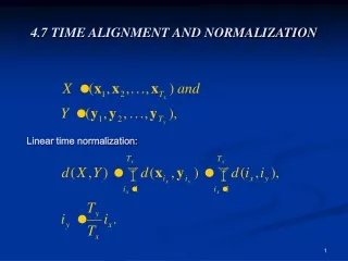
4.7 TIME ALIGNMENT AND NORMALIZATION Linear time normalization:
4.7 TIME ALIGNMENT AND NORMALIZATION m(k): a nonnegative (path) weighting factor Mϕ: a (path) normalizing factor
4.7.1 Dynamic Programming-Basic Considerations According to Bellman: An optimal policy has the property that, whatever the initial state and decisions are, the remaining decisions must constitute an optimal policy with regard to the state resulting from the first decision For every pair of points (i,j) We define to be a nonnegative cost that represents the cost of moving directly from the ith point to the jth point in one step. We are interested in obtaining the optimal sequence of moves and the associated minimum cost from any point i to any other point j in As many points as necessary.
4.7.1 Dynamic Programming-Basic Considerations To determine the minimum cost path between points i and j, the following dynamic program is used:
4.7.1 Dynamic Programming-Basic Considerations A recursion allowing the optimal path search to be conducted incrementally
4.7.1 Dynamic Programming-Basic Considerations 1- Initialization 2- Recursion
4.7.1 Dynamic Programming-Basic Considerations 3- Termination 4- Path backtracking
Time-Normalization Constraints • Endpoint constraints • Monotonicity constraints • Local continuity constraints • Global path constraints • Slope weighting
4.7.2.3 Local Continuity Constraints We define a path P as a sequence of moves, each specified by a pair of coordinate increments,
4.7.2.3 Local Continuity Constraints For a path that begins at (1,1), which point we designate k=1, we normally set (as if the path originates from (0,0)) and have:
4.7.2.4 Global Path Constraints For each type of local constraints, the allowable regions can be Defined using the following two parameters: Normally, Qmax=1/Qmin
TYPE I 0 II 2 III 2 IV 2 V 3 VI VII 3 ITAKURA 2 Values of and for different types of paths
4.7.2.4 Global Path Constraints We can define the global path constraints as follows: The first equation specifies the range of the points in the (ix, iy) plane that can be reached from the beginning point (1,1) via the allowable path according to the local constraints. The second equation specifies the range of points that have a legal path to the ending pint (Tx , Ty)
4.7.2.5 Slope Weighting The weighting function can be designed to implement an optimal discriminant analysis for improved recognition accuracy. Set of four types of slope weighting proposed by Sakoe and Chiba
4.7.2.5 Slope Weighting The Accumulated distortion also requires an overall normalization. Customarily: For type (c) and (d) slope weighting, Typically, for types (a) and (b) slope weightings, we arbitrarily set:
4.7.3 Dynamic Time-Warping Solution Due to endpoint constraints, we can write:
4.7.3 Dynamic Time-Warping Solution Similarly, the minimum partial accumulated distortion along a path Connecting (1,1) and (ix, iy) is:
4.7.3 Dynamic Time-Warping Solution The ratio of grid allowable grid points to all grid points, when a k-to-1 time scale expansion and contraction is allowed: