Download
1 / 46
460 likes | 481 Vues
Discover a new approach explaining decidability results uniformly, focusing on tree-width of graphs and MSO logic. Learn about decision problems, integer linear programming, emptiness for automata, and much more. Dive into the world of MSO formulas and bounded tree-width graphs, with applications in various areas. Explore tree decompositions, tree-width of graphs, and the satisfiability problem for MSO on different classes of graphs. Join us to uncover the hidden connections and derive new results in the realm of graph theory.

E N D
The Tree-Width of Decidable Problems Gennaro Parlato (U. Southampton, UK) joint work with: P. Madhusudan (UIUC, USA) Salvatore La Torre (U. Salerno, Italy) Constantin Enea, Peter Habermehl (LIAFA, CNRS, U. Paris 7, France) Omar Inverso (U. Southampton, UK)
what is this talk about ? A new approach that explains several decidability results in a uniform way P : decision problem search space
what is this talk about ? A new approach that explains several decidability results in a uniform way P : decision problem Integer Linear programming (ILP) x1 + x2 + … + xn = search space: N x N x … N (tuples of natural numbers) a2 an b a1 search space
what is this talk about ? A new approach that explains several decidability results in a uniform way P : decision problem Emptiness for automata: • finite state a. • pushdown a. • multi-stack a. • dist. automata with FIFO channels • … search space: init final (runs: sequences of configurations) search space
what is this talk about ? A new approach that explains several decidability results in a uniform way P : decision problem Representation depends on the problem (ILP, Empt. …) We propose uniform repr. with labeled graphs (finite set of labels) search space = class of graphs that is MSO definable (MSO=Monadic Second Order logic) search space
what is this talk about ? A new approach that explains several decidability results in a uniform way P : decision problem finding a solution to P => • exists a graph representing a solution => satisfiability of MSO on graphs Satisfibility problem for MSO • undecidable in general • decidable for bounded tree-width graphs (Courcelle/Seese’s theorem) search space
approach - MSO formula describing search space • show solutions have bounded tree-width • algorithm for free!(Courcelle’s theorem) Why • existing decision procedures intrinsically “compute” tree-decompositions • a new way to look at “old” decidable problems • derive new decidability results
outline Definitions • MSO on graphs • tree-width Applications • Emptiness automata with auxiliary storage • Integer Linear Programming Conclusions
MSO on graphs For a fixed alphabet , a -labeled graph is a structure (V, {Ea}a ) where • V is a finite set of vertices • Ea V x V is a set of edges labeled by a MSO is given by the following grammar • ::= x=y | x∈X | Ea(x,y) | ∨ | ∧ | ¬ | x. (x) | X. (X) | ∀x. (x) | ∀X. (X) where • x, y are first-order variables, X is a second-order variable • Ea(x,y) is an edge relation
MSO on graphs: examples A bipartite graph is a graph whose vertices can be divided into two disjoint sets U and V such that every edge connects a vertex in U to one in V. bipartite ≡ ∃ U,V. [ partition(U, V) ∧ ∀u,v. edge(u,v) ⇒ ((u∈U ∧ v∈V) ∨ (u∈V ∧ v∈U)) ] partition(U, V) ≡ ∀ z. (z∈U ∨ z∈V) ∧ ¬(z∈U ∧ z∈V) Graph 3-Colorability: Given an undirected graph G does there exists a way to colour the nodes red, green, and blue so that no adjacent nodes have the same colour? 3-Colorability ≡ ∃ X,Y,Z. part(X, Y, Z) ∧ ∀ u,v. (u∈X ∧ edge(u,v)) ⇒ ¬(v∈X) ∧ ∀ u,v. (u∈Y ∧ edge(u,v)) ⇒ ¬(v∈Y) ∧ ∀ u,v. (u∈Z ∧ edge(u,v)) ⇒ ¬(v∈Z)
tree-width of graphs A tree decomposition of G=(V,E) is a pair (T, {bagz }z is a node of T ), where T is a tree and bagzis a subset of G nodes, such that • every node of G is in some bag • every edge of G has both endpoints in some bag • for every node of G the set of bags that contain it form a sub-tree of T The widthof the tree decomposition is the maximum of |bagz|-1 over all T nodes z The tree-width of a graph G, is the minimum such width over all tree decompositions of G Tree width of a tree is 1
tree-decompositions (examples) 3 4 2 1 Line graph: tw=1 Cycle: tw=2 3 4 2 1 Tree: tw=1 1 Clique with k nodes: tw= k-1 2 3 4 4 7 5 6 4
MSO on graphs Satisfiability problem for MSO on a class of graphs C: • Given an MSO formula , is there a graph G in C that satisfies? • Over the class of all graphs, MSO is undecidable (even FO is undecidable) • Satisfiability problem for MSO is decidable on the class of all graphs of tree width k, for any fixed k [Courcelle/Seese’s theorem]
outline Definitions • MSO on graphs • tree-width Applications • Emptiness automata with auxiliary storage • Integer Linear Programming Conclusions ✔
Emptiness for Automata with auxiliary storage • pushdown automata • multi-stack pushdown automata • distributed automata
pushdown automata • stack S • Stack alphabet • Finite set of states Q • Initial state q1 • Final states F Q • transitions : • Internal moves: (q, q’) • Pop moves: (q, , q’) • Push moves: (q, , q’) Finite Control S
nested words (search space)(Alur-Madhusudan) A nested word NW graph captures the behavior of a run • The stack is compiled down into the nested word (nesting edges) push push push pop pop push pop pop int int int int int q7 q1 q9 q3 q11 q13 q5 q8 q2 q10 q4 q12 q6 q14 init final
nested words (search space)(Alur-Madhusudan) • The class of NWs is MSO definable • linear relation on black edges • nesting relation on matching edges • the simulation of the automaton on nested word using MSO • a second order variable for each state • a second order variable for each symbol in the stack alphabet • check internal, push, and pop moves (local check) • The class of NW has tree-width 2 (next slide) • Decidability from Courcelle’s theorem init final q7 q1 q9 q3 γ3 q11 γ11 q13 q13 q5 q8 γ2 q2 q10 γ4 q4 q12 q6 q14
1 2 3, 2, 8,13 3 14 4 9 5 7 10 6 8 11 12 13 Nested words have bounded tree-width 1 2 3 4 5 6 7 8 9 10 11 12 13 14 • Tree decomposition of NW of tw 3 • Bags: • u is un the bagu • if (u,v) is an edge of NW add u to the • bags of all nodes of the unique path • in T from u to v • captures summaries of procedures
multistack pushdown automata • Finite number of stacks S1, …,Sn • Stack alphabet • Finite set of states Q • Initial state q0 • Final states F Q • Transitions : • Internal move: (q, q’) • Pop move: (q, , stack_num, q’) • Push move: (q, , stack_num, q’) Finite Control … S1 S2 Sn
Multiply Nested Words (MNW) A MNW graph captures the behavior of a run • Stacks are compiled down into the graph (nesting edges) The class MNWs is • MSO definable • Unbounded tree-width push2 push2 pop2 pop2 int pop1 pop1 push1 push1 push1 push1 pop1 pop1
decidable emptiness problem (Madhusudan, Parlato - POPL’11) Multi-stack pushdown automata with • bounded context-switches(Rehof, Qadeer - TACAS’05) • bounded-phases(La Torre, Madhusudan, Parlato - LICS’07) • ordered(Breveglieri, Cherubini, Citrini, Crespi-Reghizzi - Int.J. Found. Comput. Sci.’95) • bounded-scope(La Torre, Napoli - CONCUR’11) (La Torre, Parlato - FSTTCS’12)
… bounded context-switches • Emptiness decidable(Qadeer, Rehof - TACAS’05) In a context only one stack can be used The class of MNWs with k contexts is • MSO definable • tree-width: k + 1
distributed automata with queues Distributed automata with queues • finite state processes • pushdown processes process FIFO channel
queue graphs (finite processes) P1: A queue graph captures the behavior of a run • queues are compiled down into the graph (blue edges) The class of queue graphs is MSO definable (linear orders for each process, FIFO edges) Unbounded tree-width P2: P3:
stack-queue graphs (PD processes) P1: • A stack-queue graph captures the behavior of a run • Stacks and queues are compiled down into the graph • The class of stack-queue graphs is MSO definable • Unbounded tree-width P2: P3:
decidable emptiness problem (POPL’11) Multi-stack pushdown automata with • bounded context-switches(Rehof, Qadeer - TACAS’05) • bounded-phases(La Torre, Madhusudan, Parlato - LICS’07) • ordered(Breveglieri, Cherubini, Citrini, Crespi-Reghizzi - Int.J. Found. Comput. Sci.’95) • Bounded-Scope(La Torre, Napoli - CONCUR’11) (La Torre, Parlato - FSTTCS’12) Distributed automata with finite processes & FIFO queues • finite state processes with polyforest architecture • pushdown processes with forest architecture + well queuing (La Torre, Madhusudan, Parlato - TACAS’08) • Non-confluent architectures + eager runs (Heußner, Leroux, Muscholl, Sutre - FOSSACS’10) (Heußner – CONCUR workshop’10)
outline Definitions • MSO on graphs • tree-width Applications • Emptiness automata • Integer Linear Programming Conclusions ✔ ✔
Integer Linear Programming (ILP) x1 + x2 + … + xn = Instance I a11 a21 . . . am1 b1 b2 . . . bm a12 a22 . . . am2 a1n a2n . . . amn SI is set of all solutions (s1,s2, …, sn) (tuple of natural numbers) Feasibility problem: is SI empty ?
plan • representing solutions with graphs rather than tuples of natural numbers • the class of all solution graphs is MSO definable • If there is a solution, there is a graph representing it of path-width 2nwhere n is the # of variables • feasibility problem reduces to the satisfiability problem of MSO on the class of 2n path-width graphs
graph representation of a solution Example 1: one constraint 3x1 – 2x2 + 1x3 = 0 solution: x1=3, x2 = 5, x3=1 x2 x1 x1 x1 x2 x2 x2 x2 x3 - + +
graph representation of a solution Example 2: (two constraints) 3x1 – 2x2 + x3 = 0 solution: x1=3, x2 = 5, x3=1 -2 x1 +1 x2 + 4 x3 = 3 constraint 1 - + + x2 x1 x1 x1 x2 x2 x2 x2 x3 b + + - - constraint 2
graph representation of a solution Solution graphs (logical characterization) is the class CIof all graphs G = (V, Lvar, {Lsigni}i in [1,…m], {Ei}i in [1,m] ) • Lvar : V -> {x1, x2, …, xn, b } with exactly one node v with Lvar(v) = b • Lsigni: V -> {+, -} - if Lvar(v) = xj then Lsigni(v) = sign( aij ) - if Lvar(v) = b then Lsigni(v) = sign( -bi ) • degreei( v ) = |aij| if Lvar(v) = xj • degreei( v ) = |bi| if Lvar(v) = b • signi(u) ≠ signi(v) if (u,v) is an edge of Ei All the above properties can be easily defined in MSO (ϕI)
Feasibility to satisfiability on graphs • Each graph G in CI corresponds to a solution: ( #nodes labeled x1, …, #nodes labeled xn ) • If s=(s1, …, sn) is a solution then there is one or more graphs G in CI s.t. G has exactly sj nodes labeled with variable xj • If s=(s1, …, sn) is a solution then there is a graph G in CI of path-width 2n representing s
bounded path-width Let s = (s1, …, sn) be a solution intuition: we construct G and its path decomposition by adding a node labeled xj in a balanced way Example: s=(x1=100, x2=50, x3=25) • each 2 (=100/50) increments of x1, increment x2 • each 4 (=100/25) increments of x1, increment x3
bounded path-width Invariant c1 ai,1 + … + cn ai,n ri = -------------------------------- smax by induction • after Increase(j) • smax • ri’ = rj + ai,j = rj + ----- ai,j = • smax • c1 ai,1 + … + (cj+smax) + … + cn ai,n • = --------------------------------------------- • smax • after Reduce • (c1 - s1) ai,1 + … + (cn- sn) • ri’= ------------------------------------= • smax s1 ai,1 + … + sn ai,n = ri - ------------------------- = ri smax Two sets of counters(initially set to 0) cj (associated to var xj) operations: - Increase(j) : cj= cj + smax - Reduce(): cj = cj – sj for all j ri (associated to i-th row of the matrix) ri = SUMj (ai,j * # increase(j))
bounded path-width Invariant c1 ai,1 + … + cn ai,n ri = -------------------------------- smax along execution of Algorithm |cj| ------- ≤ 1 smax Therefore SUM (ai,j)≤ ri ≤ SUM (ai,j) ai,j ≤0ai,j ≥0 Two sets of counters(initially set to 0) cj (associated to var xj) operations: - Increase(j) : cj= cj + smax - Reduce(): cj = cj – sj for all j ri (associated to i-th row of the matrix) ri = SUMj (ai,j * # increase(j) ) Algorithm: • Increase(max); • Reduce(), stop if ri=0 for all i • Increase(j) for all j≠max s.t. cj < 0 goto (1)
path-width decomposition - given a solution s - run algorithm according to s list of increase operations: increase( j1 ), …, increase( ji ), … increase(jt) xji xji xji xj1 add a node labeled xji -match edges -oldest nodes first -remove fully matched nodes • size of the each bag ≤ SUMi |ri| ≤ SUMi,j |ai,j| • we can prove that this path-decomposition has width at most 2n
Conclusion/Future work A general criterionthat uniformly explains many decidability results for • automata with auxiliary storage (stacks, queues) • Integer Linear Programming Other decidable results? Several decidability results for automata are obtained using Parikh + Presburger A Perfect Model for Bounded Verification [Esparza,Ganty, Majumdar, LICS’12] Is this a general principle that governs decidability?
Future work (program verification) Reasoning about Concurrent programs + Weak Memory models? Automata with heap structures? • a concurrent/distributed program can be seen as as sequential program + stacks/queues • what about lists, trees, …, graphs? Behavior graphs? Can we exploit this new view to device (under-approximate) scalable solutions for the analysis of programs??? • sequentialization of programs … tree-decompositions can be seen as a tree or a sequential programs with procedure calls • New SMT encodings (bounded model checking) • Fixed point engines …
Open problem: “abab problem” Example w = aabababbaabb[ #a(a) = #b(w)] Marking of w: aabababbaabb =w aabababbaabb(mark a) aabababbaabb(mark b) aabababbaabb(mark a) aabababbaabb(mark b) aabababbaabb(mark a) aabababbaabb(mark b) aabababbaabb(mark a) aabababbaabb(mark b) aabababbaabb(mark a) aabababbaabb(mark b) aabababbaabb(mark a) aabababbaabb(mark b) Marking Mw: row0 000000000000 row1 000100000000 row2 000100100000 row3 010100100000 row4 011100100000 row5 111100100000 row6 111100110000 row7 111100111000 row8 111110111000 row9 111111111000 row10 111111111010 row11 111111111110 row12 111111111111
Open problem: “abab problem” Let w be any word over the alphabet {a,b}, with #a(w) = #b(w). w is called balanced word. A marking of w is a bit matrix Mw of dimension (n+1) x n (rows: 0 to n) (columns: 1 to n ) • first row of M is all 0’s • for i>1, the i-th row is a copy of the (i-1)-th row except one position, say j, s. t. M[i-1, j]=0 and M[i, j]=1. Furthermore, if i is odd w[i]=a, otherwise w[i]=b
Open problem: “abab problem” Given a marking Mw of a balanced word w, we define the width of Mw as follows. The width of a row of Mw is the number of its 1-sequences. The width of Mw is the maximum width over all Mw rows. Example: The marking-width of a balanced word w, denoted marking-width(w), is the minimum width overall markings of w. Marking Mw: row0 000000000000 width = 0 row1 000100000000 width = 1 row2 000100100000 width = 2 row3 010100100000 width = 3 row4 011100100000 width = 2 row5111100100000 width = 2 row6111100110000 width = 2 row7111100111000 width = 2 row8111110111000 width = 2 row9111111111000 width = 1 row10 111111111010 width = 2 row11 111111111110 width = 1 row12 111111111111 width = 1 width(Mw)=3
Constantin Enea, Peter Habermehl, Gennaro Parlato “abab problem” Is there a constant k s. t. for every balanced word w, w has marking-width ≤ k ?