Chapter 13 Forecasting
Chapter 13 Forecasting. Topics. Components of Forecasting Time Series Methods Accuracy of Forecast Regression Methods. Components of Forecasting. Many forecasting methods are available for use Depends on the time frame and the patterns Time Frames: Short-range (one to two months)

Chapter 13 Forecasting
E N D
Presentation Transcript
Chapter 13 Forecasting
Topics • Components of Forecasting • Time Series Methods • Accuracy of Forecast • Regression Methods
Components of Forecasting • Many forecasting methods are available for use • Depends on the time frame and the patterns • Time Frames: • Short-range (one to two months) • Medium-range (two months to one or two years) • Long-range (more than one or two years) • Patterns: • Trend • Random variations • Cycles • Seasonal pattern
Forecasting Components: Patterns • Trend: A long-term movement of the item being forecast • Random variations: movements that are not predictable and follow no pattern • Cycle: A movement, up or down, that repeats itself over a time span • Seasonal pattern: Oscillating movement in demand that occurs periodically and is repetitive
Forecasting Components: Forecasting Methods • Times Series (Statistical techniques) • Uses historical data to predict future pattern • Assume that what has occurred in the past will continue to occur in the future • Based on only one factor - time. • Regression Methods • Attempts to develop a mathematical relationship between the item being forecast and the involved factors • Qualitative Methods • Uses judgment, expertise and opinion to make forecasts
Forecasting Components: Qualitative Methods • Called jury of executive opinion • Most common type of forecasting method for long-term • Performed by individuals within an organization, whose judgments and opinion are considered valid • Includes functions such as marketing, engineering, purchasing, etc. • Supported by techniques such as the Delphi Method, market research, surveys, etc.
Time Series: Techniques • Moving Average • Weighted Moving Average • Exponential Smoothing • Adjusted Exponential Smoothing • Linear Trend
Moving Average • Uses values from the recent past to develop forecasts • Smoothes out random increases and decreases • Useful for stable items (not possess any trend or seasonal pattern • Formula for:
Revisit of 3-Month and 5-Month • Longer-period moving averages react more slowly to changes in demand • Number of periods to use often requires trial-and-error experimentation • Moving average does not react well to changes (trends, seasonal effects, etc.) • Good for short-term forecasting.
Weighted Moving Average • Weights are assigned to the most recent data. • Determining precise weights and number of periods requires trial-and-error experimentation • Formula:
Exponential Smoothing: Simple Exponential Smoothing • Weights recent past data more strongly • Formula: Ft + 1 = Dt + (1 - )Ft where: Ft + 1 = the forecast for the next period Dt = actual demand in the present period Ft = the previously determined forecast for the present period = a weighting factor (smoothing constant) • Commonly used values of are between .10 and .50 • Determination of is usually judgmental and subjective
Comparing Different Smoothing Constants • Forecast that uses the higher smoothing constant (.50) reacts more strongly to changes in demand • Both forecasts lag behind actual demand • Both forecasts tend to be lower than actual demand • Recommend low smoothing constants for stable data without trend; higher constants for data with trends
Exponential Smoothing: Adjusted • Exponential smoothing with a trend adjustment factor added • Formula: A Ft + 1 = Ft + 1 + Tt+1 where: T = an exponentially smoothed trend factor Tt + 1 + (Ft + 1 - Ft) + (1 - )Tt Tt = the last period trend factor = smoothing constant for trend (between zero and one) • Weights are given to the most recent trend data and determined subjectively • Forecast is higher than the simple exponentially smooth • Useful for increasing trend of the data
Linear Trend Line • When demand displays an obvious trend over time, a linear trend line, can be used to forecast • Does not adjust to a change in the trend • Formula: Y= a+ b x
Seasonal Adjustments • Seasonal pattern is a repetitive up-and-down movement in demand • Can occur on a monthly, weekly, or daily basis. • Forecast can be developed by multiplying the normal forecast by a seasonal factor • Seasonal factor can be determined by dividing the actual demand for each seasonal period by total annual demand: • lies between zero and one Si =Di/D
Forecast Accuracy Overview • Forecasts will always deviate from actual values • Difference between forecasts and actual values referred to as forecast error • Like forecast error to be as small as possible • If error is large, either technique being used is the wrong one, or parameters need adjusting • Measures of forecast errors: • Mean Absolute deviation (MAD) • Mean absolute percentage deviation (MAPD) • Cumulative error (E bar) • Average error, or bias (E)
Forecast Accuracy: Mean Absolute Deviation • MAD is the average absolute difference between the forecast and actual demand. • Most popular and simplest-to-use measures of forecast error. • Formula: • The lower the value of MAD, the more accurate the forecast • MAD is difficult to assess by itself • Must have magnitude of the data
Mean Absolute Deviation • A variation on MAD • Measures absolute error as a percentage of demand rather than per period • Formula:
Cumulative Error • Sum of the forecast errors (E =et). • A large positive value indicates forecast is biased low • A large negative value indicates forecast is biased high • Cumulative error for trend line is always almost zero • Not a good measure for this method
Regression Methods Overview • Time series techniques relate a single variable being forecast to time. • Regression is a forecasting technique that measures the relationship of one variable to one or more other variables. • Simplest form of regression is linear regression.
Regression Methods Linear Regression • Linear regression relates demand (dependent variable ) to an independent variable.
Regression Methods: Correlation • Measure of the strength of the relationship between independent and dependent variables • Formula: • Value lies between +1 and -1. • Value of zero indicates little or no relationship between variables. • Values near 1.00 and -1.00 indicate strong linear relationship.
Regression Methods: Coefficient of Determination • Percentage of the variation in the dependent variable that results from the independent variable. • Computed by squaring the correlation coefficient, r. • If r = .948, r2 = .899 • Indicates that 89.9% of the amount of variation in the dependent variable can be attributed to the independent variable, with the remaining 10.1% due to other, unexplained, factors.
Multiple Regression • Multiple regression relates demand to two or more independent variables. General form: y = 0 + 1x1 + 2x2 + . . . + kxk where 0 = the intercept 1 . . . k = parameters representing contributions of the independent variables x1 . . . xk = independent variables