Download
1 / 24
240 likes | 336 Vues
Quantifying the organic carbon pump. Jorn Bruggeman Theoretical Biology Vrije Universiteit, Amsterdam PhD March 2004 – 2009. Contents. The project Organic carbon pump General aims Biota modeling Physics modeling New integration algorithm Criteria Mass and energy conservation

E N D
Quantifying the organic carbon pump Jorn Bruggeman Theoretical Biology Vrije Universiteit, Amsterdam PhD March 2004 – 2009
Contents • The project • Organic carbon pump • General aims • Biota modeling • Physics modeling • New integration algorithm • Criteria • Mass and energy conservation • Existing algorithms • Extended modified Patankar • Plans
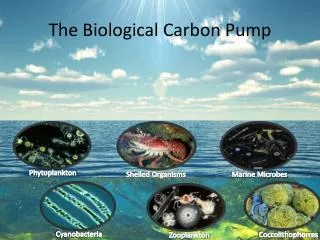
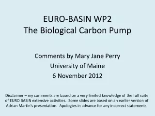
POC The biological carbon pump • Ocean top layer: CO2 consumed by phytoplankton • Phytoplankton biomass enters food web • Biomass coagulates, sinks, enters deep • Carbon from atmosphere, accumulates in deep water CO2 (g) CO2 (aq) biomass
The project • Title • “Understanding the ‘organic carbon pump’ in meso-scale ocean flows” • 3 PhDs • Physical oceanography, biology, numerical mathematics • Aim: • quantitative prediction of global organic carbon pump from 3D models • My role: • biota modeling, 1D water column
Biota modeling • Dynamic Energy Budget theory (Kooijman 2000) • Based on individual, extended to populations • Defines generic kinetics for: • food uptake • food buffering • compound conversion • reproduction, growth • Integrates existing approaches: • Michaelis-Menten functional response • Droop quota • Marr-Pirt maintenance • Von Bertalanffy growth • Body size scaling relationships
Biological model: mixotroph light CO2 DOC C-reserve death active biomass nutrient N-reserve growth detritus maintenance death
Physics modeling • GOTM water column • Open ocean test cases (less influence of horizontal advection) • weather: • light • air temperature • air pressure • relative humidity • wind speed CO2 nutrient = 0 turbulence biota carbon transport nutrient = constant
Sample results: 10 year cycle turbulence temperature biomass nutrient
Integration algorithms • (bio)chemical criteria: • Positive • Conservative • Order of accuracy • Even if model meets requirements, integration results may not
Mass and energy conservation • Model building block: transformation • Conservation • for any element, sums on left and right must be equal • Property of conservation • is independent of r • does depend on stoichiometric coefficients • Complete conservation requires preservation of stoichiometric ratios
Systems of transformations • Integration operates on (components of) ODEs • Transformation fluxes distributed over multiple ODEs:
Forward Euler, Runge-Kutta • Non-positive • Conservative (stoichiometric ratios preserved) • Order: 1, 2, 4 etc.
Backward Euler, Gear • Positive for order 1 • Conservative (stoichiometric ratios preserved) • Generalization to higher order eliminates positivity • Slow! • requires numerical approximation of partial derivatives • requires solving linear system of equations
Modified Patankar: concepts • Burchard, Deleersnijder, Meister (2003) • “A high-order conservative Patankar-type discretisation for stiff systems of production-destruction equations” • Approach • Transformation fluxes in production, destruction matrices (P, D) • Pij = rate of conversion from j to i • Dij = rate of conversion from i to j • Substrate fluxes in D, product fluxes in P
Modified Patankar: integration • Flux-specific multiplication factors cn+1/cn • Represent ratio: (substrate after) : (substrate before) • Multiple substrates in transformation: multiple, differentcn+1/cn factors • Then: stoichiometric ratios not preserved!
Modified Patankar: example and conclusion • Positive • Conservative for single-substrate transformations only! • Order 1, 2 (higher possible) • Requires solving linear system of equations
Extended Modified Patankar 1 • Non-linear system of equations • Positivity requirement fixes domain of product term p:
Extended Modified Patankar 2 • Polynomial for p: positive at left bound of p, negative at right bound • Derivative of polynomial is negative within p domain: only one valid p • Bisection technique is guaranteed to find p
Extended Modified Patankar 3 • Positive • Conservative (stoichiometric ratios preserved) • Order 1, 2 (higher should be possible) • ±20 bisection iterations (evaluations of polynomial) • Always cheaper than Backward Euler, Modified Patankar
Test case • Nitrogen + carbon phytoplankton
Plans • Publish Extended Modified Patankar • Short term • Modeling ecosystems • Aggregation into functional groups • Modeling coagulation (marine snow) • Extension to complete ocean and world; longer timescales with surfacing of deep water • GOTM in MOM/POM/…, GETM? • Integration with meso-scale eddy results