Exploring Conditional Expectation in Probability Theory
Learn about conditional expectation of discrete and continuous random variables, law of total expectation, minimum variance unbiased estimator, Rao-Blackwell Theorem, methods for finding estimators, maximum likelihood estimators, and properties of MLE.

Exploring Conditional Expectation in Probability Theory
E N D
Presentation Transcript
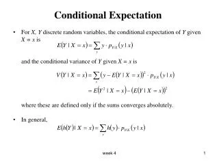
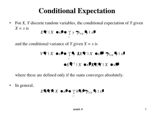
Conditional Expectation • For X, Y discrete random variables, the conditional expectation of Y given X = x is and the conditional variance of Y given X = x is where these are defined only if the sums converges absolutely. • In general, week 4
For X, Y continuous random variables, the conditional expectation of Y given X = x is and the conditional variance of Y given X = x is • In general, week 4
Example • Suppose X, Y are continuous random variables with joint density function • Find E(X | Y = 2). week 4
More about Conditional Expectation • Assume that E(Y | X = x) exists for every x in the range of X. Then, E(Y | X ) is a random variable. The expectation of this random variable is E [E(Y | X )] • Theorem E [E(Y | X )] = E(Y) This is called the “Law of Total Expectation”. Proof: week 4
Example • Suppose we roll a fair die; whatever number comes up we toss a coin that many times. What is the expected number of heads? week 4
Theorem • For random variables X, Y V(Y) = V [E(Y|X)] + E[V(Y|X)] Proof: week 4
Example • Let Y be the number of customers entering a CIBC branch in a day. It is known that Y has a Poisson distribution with some unknown mean λ. Suppose that 1% of the customers entering the branch in a day open a new CIBC bank account. • Find the mean and variance of the number of customers who open a new CIBC bank account in a day. week 4
Minimum Variance Unbiased Estimator • MVUE for θ is the unbiased estimator with the smallest possible variance. We look amongst all unbiased estimators for the one with the smallest variance. week 4
The Rao-Blackwell Theorem • Let be an unbiased estimator for θ such that . If T is a sufficient statistic for θ, define . Then, for all θ, and • Proof: week 4
How to find estimators? • There are two main methods for finding estimators: 1) Method of moments. 2) The method of Maximum likelihood. • Sometimes the two methods will give the same estimator. week 4
Method of Moments • The method of moments is a very simple procedure for finding an estimator for one or more parameters of a statistical model. • It is one of the oldest methods for deriving point estimators. • Recall: the k moment of a random variable is These will very often be functions of the unknown parameters. • The corresponding k sample moment is the average . • The estimator based on the method of moments will be the solutions to the equation μk = mk. week 4
Examples week 4
Maximum Likelihood Estimators • In the likelihood function, different values of θ will attach different probabilities to a particular observed sample. • The likelihood function, L(θ | x1, …, xn), can be maximized over θ, to give the parameter value that attaches the highest possible probability to a particular observed sample. • We can maximize the likelihood function to find an estimator of θ. • This estimator is a statistics – it is a function of the sample data. It is denoted by week 4
The log likelihood function • l(θ) = ln(L(θ)) is the log likelihood function. • Both the likelihood function and the log likelihood function have their maximums at the same value of • It is often easier to maximize l(θ). week 4
Examples week 4
Important Comment • Some MLE’s cannot be determined using calculus. This occurs whenever the support is a function of the parameter θ. • These are best solved by graphing the likelihood function. • Example: week 4
Properties of MLE • The MLE is invariant, i.e., the MLE of g(θ) equal to the function g evaluated at the MLE. • Proof: • Examples: week 4