Data sample: 130 pb - 1 (2001) + 250 pb - 1 (2002)
190 likes | 358 Vues
f f 0 g p + p - g. Data sample: 130 pb - 1 (2001) + 250 pb - 1 (2002). C. Bini S. Ventura. Spectra of 2001 and 2002 data Evaluation of luminosity and number of events Fit of the 2001+2002 spectrum Branching Ratio of f f 0 g p + p - g. Invariant Mass M pp Spectra.

Data sample: 130 pb - 1 (2001) + 250 pb - 1 (2002)
E N D
Presentation Transcript
f f0gp+p-g Data sample: 130 pb-1 (2001) + 250 pb-1 (2002) C. Bini S. Ventura • Spectra of 2001 and 2002 data • Evaluation of luminosity and number of events • Fit of the 2001+2002 spectrum • Branching Ratio of f f0g p+p-g
Invariant Mass Mpp Spectra 2002 2001
Evaluation of luminosity We have the ratio between number of events and integrated luminosity for every run: N is the number of events after selection. The mean value of R is 1.75 events per nb-1 for 2001 and 2002 data. A run is included in the evaluation of the total luminosity if R is compatible with the average.
Nrun 2001 Nrun 2002
Using the values of luminosity found we can compare the spectra of 2001 and 2002. 2001 2002
Fit of the spectra 2001+2002 The function for the fit has 4 terms: • Initial State Radiation Achasov • Final State Radiation Achasov • f f0g p+p-g Giovannella-Miscetti • Interference with Final Achasov-Giovannella-Miscetti • State Radiation We have a fit for each possible sign of the interference term.
The function for the fit depends on 9 parameters: (ds/dM)=fisr(x, mr ,Gr ,mw ,Gw , a , b) + ffsr(x, mr ,Gr ,mw ,Gw , a , b) + ff0(x, g2f0KK/4p , g2f0KK/g2f0p+p- ,mf0 ) + fint(x, g2f0KK/4p , g2f0KK/g2f0p+p- ,mf0 , mr ,Gr ,mw ,Gw , a , b) In the f0-term we replace G(f0p0p0) with: G(f0p+p-) = 2 × G(f0p0p0) e The function is multiplied by the efficiency and the luminosity: f(x) = (ds/dM) × e × T × L × DM × C T is a factor that takes into account the cut on the polar angle of the pions DM is the bin size C an overall factor : 0.8 T
Destructive Interference fisr +ffsr+ff0 -fint ALL ISR FSR f0 INT
No Interference fisr +ffsr+ff0 ALL ISR FSR f0 INT
Constructive Interference fisr +ffsr+ff0 +fint ALL ISR FSR f0 INT
For the case of destructive interference we show the variable:
Estimate of BR(f f0g p+p-g) s(f) = 3.34 mb L = 342 pb-1 Nexp( f0) is the number of ff0g events calculated integrating the contribution of the f0 to the total function without the efficiency.
Comparison with the Giovannella-Miscetti results: Giovannella – Miscetti found this value: BR(f f0g p0p0g) = (1.49 ± 0.07) ×10-4 We expect BR(f f0g p+p-g) ~ 2 ×BR(f f0g p0p0g) Instead we find: BR(f f0g p+p-g) ~ 0.58 × BR(f f0g p0p0g)
Using the parameters of Giovannella-Miscetti in the function for the fit there is not agreement with data. Constructive int. Zero int. Destructive int.
Spectrum of the data and function for different values of the photon polar angle range: The function describes quite well how the spectrum changes varying the photon polar angle range. = 25º = 45º = 65º
Fit with contribution of the s The parameterization of f (f0+s) g p+p-g is taken from Giovannella-Miscetti We include the term of interference between f s g p+p-g and the Final State Radiation. The mass and width of the s arefixed at: ms= 480 MeV Gs= 324 MeV We have only a new free parameter for the fit: gfsg
Results of the fit with the s contribution In the case of destructive interference
Conclusions • the spectrum is well described by the function in the case of • destructive interference • in the case of destructive interference we have: • without the s contribution we find: • BR(f f0g p+p-g) =8.79 × 10⁻⁵ ~0.58 × BR(f f0g p0p0g)