Download
1 / 31
320 likes | 463 Vues
}. e1-b (1999). K. Lukashin, Phys.Rev.C63:065205,2001 ( f @4.2 GeV). }. C. Hadjidakis et al., Phys.Lett.B605:256-264,2005 ( r 0 @4.2 GeV). L. Morand et al., Eur.Phys.J.A24:445-458,2005 ( w @5.75GeV). J. Santoro et al., Phys.Rev.C78:025210,2008 ( f @5.75GeV). e1-6 (2001-2002).

E N D
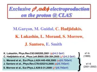
} e1-b (1999) K. Lukashin, Phys.Rev.C63:065205,2001 (f@4.2 GeV) } C. Hadjidakis et al., Phys.Lett.B605:256-264,2005 (r0@4.2 GeV) L. Morand et al., Eur.Phys.J.A24:445-458,2005 (w@5.75GeV) J. Santoro et al., Phys.Rev.C78:025210,2008 (f@5.75GeV) e1-6 (2001-2002) S. Morrow et al., Eur.Phys.J.A39:5-31,2009(r0@5.75GeV) Exclusive r0,w&f electroproduction on the proton @ CLAS M.Garçon, M. Guidal,C. Hadjidakis, K. Lukashin, L. Morand, S. Morrow, J. Santoro,E. Smith
e1-6 experiment (Ee =5.75 GeV) (October 2001 – January 2002)
Mm(epp+ X) Mm(epX) ep ep p+(p-) p+ e (p-) p
MC Acceptance calculation in 7D 200 million simulated events 100 days
ComparisonDATA-SIMULATION Naccr0+(a*NaccD++)+(b*Naccp+p-) eff = Ngenr0+(a*NgenD++)+(b*Ngenp+p-) Determine acceptance as; Determine a & b from comparison to data
BackgroundSubtraction (normalized spectra) • 1) Ross-Stodolsky B-W forr0(770),f0(980)andf2(1270) • with variable skewedness parameter, • 2)D++(1232) p+p-inv.mass spectrumandp+p- phase space.
Large tmin ! (1.6 GeV2) Fit by ebt ds/dt (g*ppr0)
Angular distribution analysis,cos qcm Relying on SCHC (exp. check to the ~25% level)
Interpretation “a la Regge” : Laget model g*p pr0 g*p pw Free parameters: *Hadronic coupling constants:gMNN *Mass scales of EM FFs:(1+Q2/L2)-2 g*p pf
sL (g*Lp prL0) s,f2 Pomeron Regge/Laget
LO (w/o kperp effect) LO (with kperp effect) Soft overlap (partial) Handbag diagram calculation has kperp effects to account for preasymptotic effects Interpretation in terms of GPDs ?
GPDs parametrization based on DDs (VGG/GK model)
VGG GPD model GK GPD model
t ERBL DGLAP x +1 -1 -ξ 0 ξ Quark distribution W~1/x γ, π, ρ, ω… -2ξ x+ξ x-ξ ~ ~ H, H, E, E (x,ξ,t) “ERBL” region “DGLAP” region Antiquark distribution q q Distributionamplitude
With : DDq(a,b)=h(a,b) q(b) h(a,b)=[(1-|b|)2-a2] and Reggeized t dependence (M.G.,Polyakov,Vanderhaeghen,Radyushkin) DDq(a,b,t)=q(b) h(a,b)b-a’(1-b)t Add new D-term in ERBL region : x Hq(x,x,t)= db da d(x-b-ax)DDq(a,b,t) +1 -1 -ξ 0 ξ +x db da d(x-b-ax)DD’(a,b,t) Which reduces to a D-term-like form as t->0 DD’(a,b,t)=a h(a,b) b’t/|b|b’t+1 With: Double Distributions parametrization (Radyushkin) Hq(x,x)~ db da d(x-b-ax)DDq(a,b) Normalization arbitrary: fitted to data!
DDs + “meson exchange” DDs w/o “meson exchange” (VGG) “meson exchange”
dsL/dt (g*ppr0) “DDs” GPDs + “meson exchange” Laget Regge
cos(qcm) distribution fcm distribution
Laget sT+esL Issue with GPD approach if p0 exchange dominant : ~ p0->E VGG esL (H&E) Laget esL while ~ E subleading in handbag for VM production Cross sections(g*p pw) LagetRegge model for g*p pw
Cross sections(g*p pw)–Comparison with GPD calculation (VGG)-
Laget sT+esL W=2.9 GeV W=2.45 GeV W=2.1 GeV GK sL fL
r w f
Summary Largest set ever of data for VM (r0,w,f) production in the valence region (sL,T, ds/dt,…) Laget Regge model describes well most of the features of (r0,w,f)cross sections (total and diff., L and T) up to Q2~3.5 GeV2. GPD handbag approach, though with large corrections (kperp), gives good description of data for W>~5 GeV for the 3 channels. For f channel: continues to work for W<~5 GeV For r channel: fails by large for W<~5 GeV (can potentially be cured by adding new contribution to GPD DD parametrisation) For w channel: fails by large for W<~5 GeV (won’t be cured by the same ansatz than the r; p0vs H&E VM GPD dominance)
GPDs/handbag ??? GPDs/handbag W~1/x