Download

1 / 27
270 likes | 290 Vues
Learn about the importance of Multi-Level Models (MLMs) in regression analysis and how they account for clustered data, such as individuals within groups or households. Discover how MLMs estimate the degree of clustering and help capture the impact of group structure on the relationship between predictors and the dependent variable.

E N D
“Multi-Level Models: What Are They and How Do They Work? ” Melinda K. Higgins, Ph.D. 30 March 2009
Why are MLM’s important? • Ordinary Least Squares (OLS) and all regression models under the General Linear Model (including logistic and poisson regression) assumes that all observations are independent of one another. • Likewise, repeated measures (time1, time2, …) assume that all time points for a given individual are independent of one another (all pairs of time points), including serial dependency (“Durbin–Watson statistic”). • When data are “clustered,” OLS may lead to inaccuracies in inference – standard errors may be too small – leads to overestimation of significance (“alpha-inflation”). • “Clusters” may include individuals within: dyads; twins; families; counseling groups; households; neighborhoods; schools; nursing units; hospitals (and repeated measures over time within an individual – the individual becomes the “cluster”).
An example • Subjects: 386 women across 40 women’s groups with a focus on diet and weight control • Group sizes range from 5-15 • Independent variable (measured for each individual) is “motivation.” • Outcome – weight loss • The groups meet regularly and may have some level of cohesion – we may expect some correlation between the individuals with a given group. • In fact, there is substantial “clustering” indicated by the fact that the groups differ substantially in average weight loss (9.75lbs-24.43lbs)
Regression – Motivation(X) vs Wt Loss (Y)(no consideration of groups)
Regression of Group Averages(avg motivation & avg weight loss) WARNING: “ECOLOGICAL FALLACY” – cannot make generalizations from the group down to the individual level. This approach only tells us the relationship between the group mean motivation and the group’s average weight loss – NOT about individuals performance.
How to estimate the “degree” of clustering?Intraclass Correlation (ICC) • The ICC measures the proportion of the total variance of an outcome variable that is accounted for by the clustering of the cases. • OLS regression (and GLM) assumes that there is no amount of variance accounted for by these “clusters”/groups; ICC=0. • ICC varies from 0 to 1 (normally). [NOTE: ICC can be negative, but it is rare – this would mean that individuals within a given “cluster” were more different from one another within the group than with individuals outside the group.] • The ICC may be initially estimated from a one-way (“Fixed Effects”) ANOVA on the groups or “clusters.” • Even for ICC’s as small as 0.01, for n=25 subjects per group, the actual alpha=0.11 (which is more than 2 times the nominal alpha=0.05). “Alpha-inflation” increases as ICC and number of subjects per group increases.
Intraclass Correlation One-Way Fixed Effects Where Mn mean number of cases per group; sd2(nj) is the variance of the number of cases per group; g=number of groups Estimated ICC=0.22 indicates substantial clustering ** [for ICC=0.20, n=10, actual alpha=0.28 not 0.05 (Kreft, deLeeuw 1998)]
“Fixed vs. Random Coefficients” OLS regression – only the outcomes and errors/residuals are considered to be random (i.e. samples from a larger population) Random Fixed “Random Coefficient” regression – now the intercepts and slopes are also considered to be RANDOM (i.e. samples from a larger population)
“Multi-Level / Hierarchical Linear Models” i=individual j=group Level 1: Individual Level; “micro-level” & Level 2: Group Level; “macro-level” Combine Level 1 and Level 2 “Additional New Parameters” – Variance Components – help to capture the impact of the group structure on the relationship of the predictors on the dependent variable.
Unconditional Cell Means Model Calculate ICC from the RC model using only the group membership (no level 1 predictor) – equivalent to a “One-way Random Effects ANOVA” = MIXED pounds BY group /CRITERIA=CIN(95) MXITER(100) MXSTEP(5) SCORING(1) SINGULAR(0.000000000001) HCONVERGE(0, ABSOLUTE) LCONVERGE(0, ABSOLUTE) PCONVERGE(0.000001, ABSOLUTE) /FIXED=| SSTYPE(3) /METHOD=REML /PRINT=CPS CORB COVB DESCRIPTIVES G LMATRIX R SOLUTION TESTCOV /RANDOM=INTERCEPT | SUBJECT(group) COVTYPE(UN) /EMMEANS=TABLES(OVERALL). [for ICC=0.20, n=10, actual alpha=0.28 not 0.05 (Kreft, deLeeuw 1998)]
Unconditional Cell Means Model = = 16.069 is significant (pval<0.001) – 16.069 units of within class variance in pounds lost that might be significantly accounted for by motivation predictors. = 4.906 is also significant (pval=0.002) – 4.906 units of between class variance in pounds lost (reflects differences between groups in mean pounds lost); and since this is significantly > 0, indicates that there is random variation among the intercepts of the various groups – WE SHOULD NOT IGNORE CLUSTERING.
Random Coefficient Model Mixed Level 1 & 2 MIXED pounds BY group WITH motivatc /CRITERIA=CIN(95) MXITER(100) MXSTEP(5) SCORING(1) SINGULAR(0.000000000001) HCONVERGE(0, ABSOLUTE) LCONVERGE(0, ABSOLUTE) PCONVERGE(0.000001, ABSOLUTE) /FIXED=motivatc | SSTYPE(3) /METHOD=REML /PRINT=CPS CORB COVB DESCRIPTIVES G LMATRIX R SOLUTION TESTCOV /RANDOM=INTERCEPT motivatc | SUBJECT(group) COVTYPE(UN) /EMMEANS=TABLES(OVERALL). Level 2 Level 1
Consider the Fixed EffectsPortion of the Model Fixed Random Weight Loss (Yij) = 15.137701 lbs + 3.118 units_motivation/lbs *(motivation_ctr (xij)) Both the intercept and slope are significant (both pval<0.001). So, for every unit increase in motivation, 3.118 more lbs are lost; with an average weight loss per group of 15.14 lbs.
Consider the Random EffectPortion of the Model variance of the slopes across groups is significant (again do not ignore clustering) the covariance between slopes and intercepts was positive indicating the higher the average pounds lost in a group (intercept), the stronger the positive relationship of motivation on weight loss; but this was not significant. the addition of motivation as a predictor reduced the within group variance in pounds lost by 63% (from 16.069 to 5.933) the addition of motivation as a predictor also reduced the between group differences in avg. pounds lost (intercepts) by 51% (4.906 to 2.397) SO, overall there were fluctuations between the groups in terms of mean pounds lost – these fluctuations were systematically related to the mean motivation level of individuals within these groups. Cannot test this via ANCOVA nor (g-1) dummy variables in regression.
MLM with Predictor at Level 2 (group variable)“treatment” = diet program vs control Fixed Random MIXED pounds BY group WITH motivatc treatc /CRITERIA=CIN(95) MXITER(100) MXSTEP(5) SCORING(1) SINGULAR(0.000000000001) HCONVERGE(0, ABSOLUTE) LCONVERGE(0, ABSOLUTE) PCONVERGE(0.000001, ABSOLUTE) /FIXED=motivatc treatc motivatc*treatc | SSTYPE(3) /METHOD=REML /PRINT=CPS CORB COVB DESCRIPTIVES G LMATRIX R SOLUTION TESTCOV /RANDOM=INTERCEPT motivatc | SUBJECT(group) COVTYPE(UN) /EMMEANS=TABLES(OVERALL).
Repeated Measures Investigate the following hypothetical data set. YA is the outcome measures over 5 time points for 60 individuals
YA-Model 1(random intercept – cell means model) = MIXED YA BY ID /CRITERIA=CIN(95) MXITER(100) MXSTEP(5) SCORING(1) SINGULAR(0.000000000001) HCONVERGE(0, ABSOLUTE) LCONVERGE(0, ABSOLUTE) PCONVERGE(0.000001, ABSOLUTE) /FIXED=| SSTYPE(3) /METHOD=REML /PRINT=CPS CORB COVB DESCRIPTIVES G LMATRIX R SOLUTION TESTCOV /RANDOM=INTERCEPT | SUBJECT(ID) COVTYPE(UN) /EMMEANS=TABLES(OVERALL). DO NOT IGNORE CLUSTERING
YA-Model 3(random intercept and slope & fixed time) i=time; j=individual MIXED YA BY ID WITH TIME /CRITERIA=CIN(95) MXITER(100) MXSTEP(5) SCORING(1) SINGULAR(0.000000000001) HCONVERGE(0, ABSOLUTE) LCONVERGE(0, ABSOLUTE) PCONVERGE(0.000001, ABSOLUTE) /FIXED=TIME | SSTYPE(3) /METHOD=REML /PRINT=CPS CORB COVB DESCRIPTIVES G LMATRIX R SOLUTION TESTCOV /RANDOM=INTERCEPT TIME | SUBJECT(ID) COVTYPE(UN) /EMMEANS=TABLES(OVERALL).
Notes on the MLM approach to RM-ANOVAfor YA – Model 3 • Model 3 added “time” as a fixed predictor to the model to determine whether there was a significant “linear” effect of time. • There is a significant effect of adding time to the model ( residual error dropped from 3.02 down to 0.228), which is still significant. • Adding time to the model also accounted for all the significant variance in the slopes of YA on time, e.g. differences between slopes were no longer significant (pval = 0.140). And the covariance (between slopes and intercepts) is also not significant. • Individual mean differences (intercepts) (pval<0.001) remain a significant source of variance.
Summary • If you suspect group (or cluster) effects, i.e. subjects within your groups may exhibit some level of “cohesion” or “alikeness,” leading you to think they are more alike within groups than between groups, the ICC should be calculated and evaluated. • If ICC is close to 0, run both OLS regression and a Random Coefficient (“mixed”) model and compare. Evaluate the “random variance components.” • Try comparing RM-ANOVA with the “mixed” multi-level model approach where “time” is level 1 and the individual is level 2. Evaluate the impact of adding time to the model.
References • Cohen, Jacob; Cohen, Patricia; West, Stephen; Aiken, Leona. “Applied Multiple Regression/Correlation Analysis for the Behavioral Sciences” 3rd edition, Lawrence Erlbaum Associates Inc., 2003. • [All data/examples in this lecture came from this book – • mostly Chapter 14 (Randon Coefficient Regression and Multilevel Models) and • Section 15.4 (Multilevel Regression of Individual Changes Over Time)] • Raudenbush; Stephen W.; Bryk, Anthony S. “Hierarchical Linear Models: Applications and Data Analysis Methods” 2nd edition, SAGE publications, 2002. • Kreft, Ita; de Leeuw, Jan. “Introducing Multilevel Modeling,” SAGE publications, 1998. • Tabachnick, Barbara G.; Fidell, Linda S. “Using Multivariate Statistics,” 5th edition, Pearson Education Inc., 2007. [Chapter 15 focuses on Multilevel Linear Modeling.] *
SON S:\Shared\Statistics_MKHiggins\website2\index.htm [updates in process] Working to include tip sheets (for SPSS, SAS, and other software), lectures (PPTs and handouts), datasets, other resources and references Statistics At Nursing Website: [website being updated] http://www.nursing.emory.edu/pulse/statistics/ And Blackboard Site (in development) for “Organization: Statistics at School of Nursing” Contact Dr. Melinda Higgins Melinda.higgins@emory.edu Office: 404-727-5180 / Mobile: 404-434-1785 VIII. Statistical Resources and Contact Info