Ways to Circumvent Time Constraints
150 likes | 184 Vues
Large-scale atmospheric circulations with Rossby waves require overcoming time constraints to simulate accurately. Learn about circumventing limitations with filtered equations, using implicit schemes, and mixed schemes for gravity waves.

Ways to Circumvent Time Constraints
E N D
Presentation Transcript
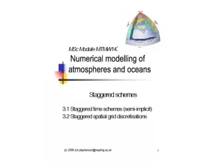
Most physically significant large-scale atmospheric circulations have time scales on the order of Rossby waves but much larger than the time scales of gravity waves. The maximum stable time step determined from the CFL condition for gravity waves is much less than that to accurately simulate the relevant phenomena.
Ways to Circumvent Time Constraints • Approximate the full governing equations with a “filtered” set of equations. • Primitive Equations • Euler Equations • Vorticity Eqns with Geostrophic Approx. • Use numerical techniques to stabilize the fast-moving waves. Generally, accuracy of the fast waves is sacrificed for efficiency.
Implicit Schemes Discretize: Center the time-derivative and choose level for RHS. Explicit: The same equation with 2x the time step gives the more common form of an explicit scheme. Implicit: Most often use some combination of the two schemes => Semi-Implicit
Example: Diffusion Assume that the diffusion coefficient is constant. Explicit: von Neumann => Stability Constraint =>
Example: Diffusion Implicit: This system can be solved by inverting the tridiagonal matrix. Using the boundary conditions to solve backwards in time! Often fully implicit schemes are too difficult to invert efficiently. von Neumann Stability => => Unconditionally stable A1 for all ∆t>0. => Only first order accurate.
Example: Diffusion Semi-Implicit Scheme: A combination of the implicit and explicit. Crank-Nicholson Scheme von Neumann Stability => => Unconditionally Stable AND accurate.
Notes on Using Implicit Schemes • Higher order implicit schemes are not necessarily more stable than the related explicit methods. • Example: the 3rd and 4th order Adams-Moulton schemes (Backward and Trapezoid are the 1st and 2nd order of this family) generally amplify solutions for any choice of time step. • Generally, only use implicit schemes for those terms that are crucial to fast waves. Use explicit methods on all other terms.
Split into Baroclinic and Barotropic modes. Rossby wave = Low Frequency Gravity wave = High Frequency
Mixed Schemes Trapezoid method. Stable when the mean flow, U, < gravity wave speed, the fluid depth, H, > the wave perturbations and the CFL condition for the Rossby wave is satisfied. These conditions are not always satisfied in the polar regions of the Earth’s atmosphere. Here, the averaging can occur in a couple different ways: The trapezoid method as above. The longer time step can be subdivided into M smaller steps ∆t/M, iterated only for the gravity wave term and then averaged over the longer time step. Note: the gravity wave term is slowed down for this calculation.
LeVeque: Finite Difference Methods for Ordinary and Partial Differential Equations; SIAM, 2007.