Download
1 / 43
430 likes | 588 Vues
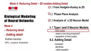
Week 4 : Reducing Detail – 2D models-Adding Detail. 3 .1 From Hodgkin-Huxley to 2D 3 .2 Phase Plane Analysis 3 .3 Analysis of a 2D Neuron Model 4 .1 Type I and II Neuron Models - limit cycles - where is the firing threshold ? - separation of time scales

E N D
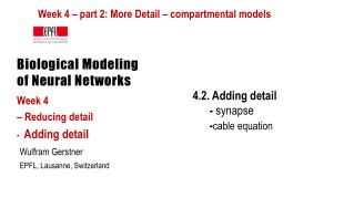
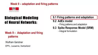
Week 4: Reducing Detail – 2D models-Adding Detail 3.1 From Hodgkin-Huxley to 2D 3.2 Phase Plane Analysis 3.3 Analysis of a 2D NeuronModel 4.1 Type I and II NeuronModels - limit cycles • - whereis the firingthreshold? - separation of time scales 4.2. AddingDetail - synapses -dendrites - cableequation Biological Modelingof Neural Networks Week 4 – Reducing detail - Adding detail Wulfram Gerstner EPFL, Lausanne, Switzerland
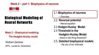
Neuronal Dynamics – Review from week 3 • Reduction of Hodgkin-Huxley to 2 dimension • -step 1: separation of time scales • -step 2: exploit similarities/correlations
Neuronal Dynamics – 4.1. Reduction of Hodgkin-Huxley model 2) dynamics of h and nare similar w(t) w(t) 1) dynamics of mare fast
stimulus Neuronal Dynamics – 4.1. Analysis of a 2D neuron model 2-dimensional equation w Enables graphical analysis! I(t)=I0 u • Pulse input • AP firing (or not) • Constant input • repetitive firing (or not) • limit cycle (or not)
Week 4 – part 1: Reducing Detail – 2D models 3.1 From Hodgkin-Huxley to 2D 3.2 Phase Plane Analysis 3.3 Analysis of a 2D NeuronModel 4.1 Type I and II NeuronModels - limit cycles • - whereis the firingthreshold? - separation of time scales 4.2. Dendrites ramp input/ constant input neuron I0 Type I and type II models f-I curve f-I curve f I0 I0
Neuronal Dynamics – 4.1. Type I and II Neuron Models neuron ramp input/ constant input I0 Type I and type II models f-I curve f-I curve f I0 I0
stimulus 2 dimensional Neuron Models w-nullcline w I(t)=I0 apply constant stimulus I0 u u-nullcline
stimulus FitzHughNagumo Model – limit cycle w I(t)=I0 -unstablefixed point -closedboundary witharrowspointinginside u limit cycle limit cycle
Neuronal Dynamics – 4.1. Limit Cycle -unstable fixed point in 2D -bounding box with inward flow limit cycle (Poincare Bendixson) Image: Neuronal Dynamics, Gerstner et al., Cambridge Univ. Press (2014)
Neuronal Dynamics – 4.1. Limit Cycle In 2-dimensional equations, a limit cycle must exist, if we can find a surface -containing one unstable fixed point -no other fixed point -bounding box with inward flow limit cycle (Poincare Bendixson) Image: Neuronal Dynamics, Gerstner et al., Cambridge Univ. Press (2014)
stimulus Discontinuous gain function Type II Model constant input w Hopf bifurcation I(t)=I0 u I0 Stabilitylost oscillation withfinitefrequency
Discontinuous gain function: Type II Neuronal Dynamics – 4.1. Hopf bifurcation: f-I -curve f-I curve ramp input/ constant input I0 I0 Stabilitylost oscillation withfinitefrequency
Neuronal Dynamics – 4.1,Type I and II Neuron Models neuron ramp input/ constant input I0 Now: Type I model Type I and type II models f-I curve f-I curve f I0 I0
stimulus Neuronal Dynamics – 4.1. Type I and II Neuron Models type I Model: 3 fixed points size of arrows! w apply constant stimulus I0 I(t)=I0 u Saddle-node bifurcation unstable saddle stable
stimulus Saddle-node bifurcation w Blackboard: - flow arrows, - ghost/ruins I(t)=I0 u unstable saddle stable
stimulus Low-frequencyfiring type I Model – constant input w I(t)=I0 u I0
stimulus Low-frequencyfiring type I Model – Morris-Lecar: constant input w I(t)=I0 u I0
Type I and type II models Response at firing threshold? Type I type II Saddle-Node Onto limit cycle For example: Subcritical Hopf ramp input/ constant input f-I curve f-I curve f f I0 I0 I0
Neuronal Dynamics – 4.1. Type I and II Neuron Models neuron ramp input/ constant input I0 Type I and type II models f-I curve f-I curve f I0 I0
Neuronal Dynamics – Quiz 4.1. 2-dimensional neuron model with (supercritical) saddle-node-onto-limit cycle bifurcation [ ] The neuron model is of type II, because there is a jump in the f-I curve [ ] The neuron model is of type I, because the f-I curve is continuous [ ] The neuron model is of type I, if the limit cycle passes through a regime where the flow is very slow. [ ] in the regime below the saddle-node-onto-limit cycle bifurcation, the neuron is at rest or will converge to the resting state. B. Threshold in a 2-dimensional neuron model with subcritical Hopf bifurcation [ ] The neuron model is of type II, because there is a jump in the f-I curve [ ] The neuron model is of type I, because the f-I curve is continuous [ ] in the regime below the Hopf bifurcation, the neuron is at rest or will necessarily converge to the resting state
Week 4 – part 1: Reducing Detail – 2D models 3.1 From Hodgkin-Huxley to 2D 3.2 Phase Plane Analysis 3.3 Analysis of a 2D NeuronModel 4.1 Type I and II NeuronModels - limit cycles • - whereis the firingthreshold? - separation of time scales 4.2. Addingdetail Biological Modelingof Neural Networks Week 4 – Reducing detail - Adding detail Wulfram Gerstner EPFL, Lausanne, Switzerland
Neuronal Dynamics – 4.1. Threshold in 2dim. Neuron Models neuron pulse input I(t) Delayed spike u Reduced amplitude u
Neuronal Dynamics – 4.1 Bifurcations, simplifications Bifurcations in neural modeling, Type I/II neuron models, Canonical simplified models Nancy Koppell, Bart Ermentrout, John Rinzel, Eugene Izhikevich and many others
stimulus Review: Saddle-node onto limit cycle bifurcation w I(t)=I0 u unstable saddle stable
stimulus Neuronal Dynamics – 4.1 Pulse input w pulse input I(t)=I0 u I(t) unstable saddle stable
stimulus 4.1 Type I model: Pulse input saddle w pulse input Slow! u I(t) blackboard Threshold for pulse input
4.1 Type I model: Threshold for Pulse input Stable manifold plays role of ‘Threshold’ (for pulse input) Image: Neuronal Dynamics, Gerstner et al., Cambridge Univ. Press (2014)
4.1 Type I model: Delayed spike initation for Pulse input Delayed spike initiation close to ‘Threshold’ (for pulse input) Image: Neuronal Dynamics, Gerstner et al., Cambridge Univ. Press (2014)
Neuronal Dynamics – 4.1 Threshold in 2dim. Neuron Models neuron pulse input I(t) Reduced amplitude Delayed spike u u NOW: model with subc. Hopf
Review: FitzHugh-Nagumo Model: Hopf bifurcation stimulus w-nullcline w I(t)=I0 apply constant stimulus I0 u u-nullcline
FitzHugh-NagumoModel - pulse input stimulus Stable fixed point w No explicit threshold for pulse input pulse input I(t) u I(t)=0
Week 4 – part 1: Reducing Detail – 2D models 3.1 From Hodgkin-Huxley to 2D 3.2 Phase Plane Analysis 3.3 Analysis of a 2D NeuronModel 4.1 Type I and II NeuronModels - limit cycles • - whereis the firingthreshold? - separation of time scales 4.2. Dendrites Biological Modelingof Neural Networks Week 4 – Reducing detail - Adding detail Wulfram Gerstner EPFL, Lausanne, Switzerland
FitzHugh-Nagumo Model - pulse input threshold? stimulus Stable fixed point w Separation of time scales pulse input I(t)=0 I(t) u blackboard
4.1 FitzHugh-Nagumo model: Threshold for Pulse input Assumption: Middle branch of u-nullcline plays role of ‘Threshold’ (for pulse input) Image: Neuronal Dynamics, Gerstner et al., Cambridge Univ. Press (2014)
stimulus 4.1 Detour: Separation fo time scales in 2dim models Assumption: Image: Neuronal Dynamics, Gerstner et al., Cambridge Univ. Press (2014)
4.1 FitzHugh-Nagumo model: Threshold for Pulse input Assumption: slow fast slow slow fast slow trajectory -follows u-nullcline: -jumps between branches: slow Image: Neuronal Dynamics, Gerstner et al., Cambridge Univ. Press (2014) fast
Neuronal Dynamics – 4.1 Threshold in 2dim. Neuron Models neuron pulse input I(t) Biological input scenario Mathematical explanation: Graphical analysis in 2D Reduced amplitude Delayed spike u u
Exercise 1: NOW! inhibitory rebound Assume separation of time scales w I(t)=0 Stable fixed point at -I0 u I(t)=I0<0 0 Next lecture: 10:55 -I0 I(t)
Neuronal Dynamics – Literature for week 3 and 4.1 Reading: W. Gerstner, W.M. Kistler, R. Naud and L. Paninski, Neuronal Dynamics: from single neurons to networks and models of cognition. Chapter 4: Introduction. Cambridge Univ. Press, 2014 OR W. Gerstner and W.M. Kistler, Spiking Neuron Models, Ch.3. Cambridge 2002 OR J. Rinzel and G.B. Ermentrout, (1989). Analysis of neuronal excitability and oscillations. In Koch, C. Segev, I., editors, Methods in neuronal modeling. MIT Press, Cambridge, MA. • Selectedreferences. • -Ermentrout, G. B. (1996). Type I membranes, phase resetting curves, and synchrony. • Neural Computation, 8(5):979-1001. • Fourcaud-Trocme, N., Hansel, D., van Vreeswijk, C., and Brunel, N. (2003). How spike generation mechanisms determine the neuronal response to fluctuating input. • J. Neuroscience, 23:11628-11640. • Badel, L., Lefort, S., Berger, T., Petersen, C., Gerstner, W., and Richardson, M. (2008). Biological Cybernetics, 99(4-5):361-370. • - E.M. Izhikevich, Dynamical Systems in Neuroscience, MIT Press (2007)
Neuronal Dynamics – Quiz 4.2. Threshold in a 2-dimensional neuron model with saddle-node bifurcation [ ] The voltage threshold for repetitive firing is always the same as the voltage threshold for pulse input. [ ] in the regime below the saddle-node bifurcation, the voltage threshold for repetitive firing is given by the stable manifold of the saddle. [ ] in the regime below the saddle-node bifurcation, the voltage threshold for repetitive firing is given by the middle branch of the u-nullcline. [ ] in the regime below the saddle-node bifurcation, the voltage threshold for action potential firing in response to a short pulse input is given by the middle branch of the u-nullcline. [ ] in the regime below the saddle-node bifurcation, the voltage threshold for action potential firing in response to a short pulse input is given by the stable manifold of the saddle point. B. Threshold in a 2-dimensional neuron model with subcritical Hopf bifurcation [ ]in the regime below the bifurcation, the voltage threshold for action potential firing in response to a short pulse input is given by the stable manifold of the saddle point. [ ] in the regime below the bifurcation, a voltage threshold for action potential firing in response to a short pulse input exists only if