Download
1 / 47
480 likes | 534 Vues
Learn about the trends in microprocessor architectures, limitations of memory system performance, and the impact of memory latency and bandwidth on parallel computing platforms. Discover how caches can improve effective memory latency.

E N D
Share Memory Systems and Message Passing Systems Taken from:Parallel Computing Platforms, byAnanth Grama, Anshul Gupta, George Karypis, and Vipin Kumar To accompany the text ``Introduction to Parallel Computing'', Addison Wesley, 2003.
Topic Overview • Implicit Parallelism: Trends in Microprocessor Architectures • Limitations of Memory System Performance • Dichotomy of Parallel Computing Platforms • Communication Model of Parallel Platforms • Case Studies
Scope of Parallelism • Conventional architectures coarsely comprise of a processor, memory system, and the data path. • Each of these components present significant performance bottlenecks. • Parallelism addresses each of these components in significant ways. • Different applications utilize different aspects of parallelism - e.g., data intensive applications utilize high aggregate throughput, server applications utilize high aggregate network bandwidth, and scientific applications typically utilize high processing and memory system performance. • It is important to understand each of these performance bottlenecks.
Implicit Parallelism: Trends in Microprocessor Architectures • Microprocessor clock speeds have posted impressive gains over the past two decades (two to three orders of magnitude). • Higher levels of device integration have made available a large number of transistors. • The question of how best to utilize these resources is an important one. • Current processors use these resources in multiple functional units and execute multiple instructions in the same cycle. • The precise manner in which these instructions are selected and executed provides impressive diversity in architectures.
Limitations of Memory System Performance • Memory system, and not processor speed, is often the bottleneck for many applications. • Memory system performance is largely captured by two parameters, latency and bandwidth. • Latency is the time from the issue of a memory request to the time the data is available at the processor. • Bandwidth is the rate at which data can be pumped to the processor by the memory system.
Memory System Performance: Bandwidth and Latency • It is very important to understand the difference between latency and bandwidth. • Consider the example of a fire-hose. If the water comes out of the hose two seconds after the hydrant is turned on, the latency of the system is two seconds. • Once the water starts flowing, if the hydrant delivers water at the rate of 5 gallons/second, the bandwidth of the system is 5 gallons/second. • If you want immediate response from the hydrant, it is important to reduce latency. • If you want to fight big fires, you want high bandwidth.
Memory Latency: An Example • Consider a processor operating at 1 GHz (1 ns clock) connected to a DRAM with a latency of 100 ns (no caches). Assume that the processor has two multiply-add units and is capable of executing four instructions in each cycle of 1 ns. The following observations follow: • The peak processor rating is 4 GFLOPS. • Since the memory latency is equal to 100 cycles and block size is one word, every time a memory request is made, the processor must wait 100 cycles before it can process the data.
Memory Latency: An Example • On the above architecture, consider the problem of computing a dot-product of two vectors. • A dot-product computation performs one multiply-add on a single pair of vector elements, i.e., each floating point operation requires one data fetch. • It follows that the peak speed of this computation is limited to one floating point operation every 100 ns, or a speed of 10 MFLOPS, a very small fraction of the peak processor rating!
Improving Effective Memory Latency Using Caches • Caches are small and fast memory elements between the processor and DRAM. • This memory acts as a low-latency high-bandwidth storage. • If a piece of data is repeatedly used, the effective latency of this memory system can be reduced by the cache. • The fraction of data references satisfied by the cache is called the cache hit ratio of the computation on the system. • Cache hit ratio achieved by a code on a memory system often determines its performance.
Impact of Caches: Example Consider the architecture from the previous example. In this case, we introduce a cache of size 32 KB with a latency of 1 ns or one cycle. We use this setup to multiply two matrices A and B of dimensions 32 × 32. We have carefully chosen these numbers so that the cache is large enough to store matrices A and B, as well as the result matrix C.
Impact of Caches: Example (continued) • The following observations can be made about the problem: • Fetching the two matrices into the cache corresponds to fetching 2K words, which takes approximately 200 µs. • Multiplying two n × n matrices takes 2n3 operations. For our problem, this corresponds to 64K operations, which can be performed in 16K cycles (or 16 µs) at four instructions per cycle. • The total time for the computation is therefore approximately the sum of time for load/store operations and the time for the computation itself, i.e., 200 + 16 µs. • This corresponds to a peak computation rate of 64K/216 or 303 MFLOPS.
Impact of Caches • Repeated references to the same data item correspond to temporal locality. • In our example, we had O(n2) data accesses and O(n3) computation. This asymptotic difference makes the above example particularly desirable for caches. • Data reuse is critical for cache performance.
Impact of Memory Bandwidth • Memory bandwidth is determined by the bandwidth of the memory bus as well as the memory units. • Memory bandwidth can be improved by increasing the size of memory blocks. • The underlying system takes l time units (where l is the latency of the system) to deliver b units of data (where b is the block size).
Impact of Memory Bandwidth: Example • Consider the same setup as before, except in this case, the block size is 4 words instead of 1 word. We repeat the dot-product computation in this scenario: • Assuming that the vectors are laid out linearly in memory, eight FLOPs (four multiply-adds) can be performed in 200 cycles. • This is because a single memory access fetches four consecutive words in the vector. • Therefore, two accesses can fetch four elements of each of the vectors. This corresponds to a FLOP every 25 ns, for a peak speed of 40 MFLOPS.
Impact of Memory Bandwidth • It is important to note that increasing block size does not change latency of the system. • Physically, the scenario illustrated here can be viewed as a wide data bus (4 words or 128 bits) connected to multiple memory banks. • In practice, such wide buses are expensive to construct. • In a more practical system, consecutive words are sent on the memory bus on subsequent bus cycles after the first word is retrieved.
Impact of Memory Bandwidth • The above examples clearly illustrate how increased bandwidth results in higher peak computation rates. • The data layouts were assumed to be such that consecutive data words in memory were used by successive instructions (spatial locality of reference). • If we take a data-layout centric view, computations must be reordered to enhance spatial locality of reference.
Impact of Memory Bandwidth: Example Consider the following code fragment: for (i = 0; i < 1000; i++) column_sum[i] = 0.0; for (j = 0; j < 1000; j++) column_sum[i] += b[j][i]; The code fragment sums columns of the matrix b into a vectorcolumn_sum.
Impact of Memory Bandwidth: Example • The vector column_sum is small and easily fits into the cache • The matrix b is accessed in a column order. • The strided access results in very poor performance. Multiplying a matrix with a vector: (a) multiplying column-by-column, keeping a running sum; (b) computing each element of the result as a dot product of a row of the matrix with the vector.
Impact of Memory Bandwidth: Example We can fix the above code as follows: for (i = 0; i < 1000; i++) column_sum[i] = 0.0; for (j = 0; j < 1000; j++) for (i = 0; i < 1000; i++) column_sum[i] += b[j][i]; In this case, the matrix is traversed in a row-order and performance can be expected to be significantly better.
Memory System Performance: Summary • The series of examples presented in this section illustrate the following concepts: • Exploiting spatial and temporal locality in applications is critical for amortizing memory latency and increasing effective memory bandwidth. • The ratio of the number of operations to number of memory accesses is a good indicator of anticipated tolerance to memory bandwidth. • Memory layouts and organizing computation appropriately can make a significant impact on the spatial and temporal locality.
Alternate Approaches for Hiding Memory Latency • Consider the problem of browsing the web on a very slow network connection. We deal with the problem in one of three possible ways: • we anticipate which pages we are going to browse ahead of time and issue requests for them in advance; • we open multiple browsers and access different pages in each browser, thus while we are waiting for one page to load, we could be reading others; or • we access a whole bunch of pages in one go - amortizing the latency across various accesses. • The first approach is called prefetching, the second multithreading, and the third one corresponds to spatial locality in accessing memory words.
Multithreading for Latency Hiding A thread is a single stream of control in the flow of a program. We illustrate threads with a simple example: for (i = 0; i < n; i++) c[i] = dot_product(get_row(a, i), b); Each dot-product is independent of the other, and therefore represents a concurrent unit of execution. We can safely rewrite the above code segment as: for (i = 0; i < n; i++) c[i] = create_thread(dot_product,get_row(a, i), b);
Multithreading for Latency Hiding: Example • In the code, the first instance of this function accesses a pair of vector elements and waits for them. • In the meantime, the second instance of this function can access two other vector elements in the next cycle, and so on. • After l units of time, where l is the latency of the memory system, the first function instance gets the requested data from memory and can perform the required computation. • In the next cycle, the data items for the next function instance arrive, and so on. In this way, in every clock cycle, we can perform a computation.
Multithreading for Latency Hiding • The execution schedule in the previous example is predicated upon two assumptions: the memory system is capable of servicing multiple outstanding requests, and the processor is capable of switching threads at every cycle. • It also requires the program to have an explicit specification of concurrency in the form of threads. • Machines such as the HEP and Tera rely on multithreaded processors that can switch the context of execution in every cycle. Consequently, they are able to hide latency effectively.
Prefetching for Latency Hiding • Misses on loads cause programs to stall. • Why not advance the loads so that by the time the data is actually needed, it is already there! • The only drawback is that you might need more space to store advanced loads. • However, if the advanced loads are overwritten, we are no worse than before!
Tradeoffs of Multithreading and Prefetching • Multithreading and prefetching are critically impacted by the memory bandwidth. Consider the following example: • Consider a computation running on a machine with a 1 GHz clock, 4-word cache line, single cycle access to the cache, and 100 ns latency to DRAM. The computation has a cache hit ratio at 1 KB of 25% and at 32 KB of 90%. Consider two cases: first, a single threaded execution in which the entire cache is available to the serial context, and second, a multithreaded execution with 32 threads where each thread has a cache residency of 1 KB. • If the computation makes one data request in every cycle of 1 ns, you may notice that the first scenario requires 400MB/s of memory bandwidth and the second, 3GB/s.
Tradeoffs of Multithreading and Prefetching • Bandwidth requirements of a multithreaded system may increase very significantly because of the smaller cache residency of each thread. • Multithreaded systems become bandwidth bound instead of latency bound. • Multithreading and prefetching only address the latency problem and may often exacerbate the bandwidth problem. • Multithreading and prefetching also require significantly more hardware resources in the form of storage.
Dichotomy of Parallel Computing Platforms • An explicitly parallel program must specify concurrency and interaction between concurrent subtasks. • The former is sometimes also referred to as the control structure and the latter as the communication model.
Control Structure of Parallel Programs • Parallelism can be expressed at various levels of granularity - from instruction level to processes. • Between these extremes exist a range of models, along with corresponding architectural support.
Control Structure of Parallel Programs • Processing units in parallel computers either operate under the centralized control of a single control unit or work independently. • If there is a single control unit that dispatches the same instruction to various processors (that work on different data), the model is referred to as single instruction stream, multiple data stream (SIMD). • If each processor has its own control control unit, each processor can execute different instructions on different data items. This model is called multiple instruction stream, multiple data stream (MIMD).
SIMD and MIMD Processors A typical SIMD architecture (a) and a typical MIMD architecture (b).
SIMD Processors • Some of the earliest parallel computers such as the Illiac IV, MPP, DAP, CM-2, and MasPar MP-1 belonged to this class of machines. • Variants of this concept have found use in co-processing units such as the MMX units in Intel processors and DSP chips such as the Sharc. • SIMD relies on the regular structure of computations (such as those in image processing). • It is often necessary to selectively turn off operations on certain data items. For this reason, most SIMD programming paradigms allow for an ``activity mask'', which determines if a processor should participate in a computation or not.
Conditional Execution in SIMD Processors Executing a conditional statement on an SIMD computer with four processors: (a) the conditional statement; (b) the execution of the statement in two steps.
MIMD Processors • In contrast to SIMD processors, MIMD processors can execute different programs on different processors. • A variant of this, called single program multiple data streams (SPMD) executes the same program on different processors. • It is easy to see that SPMD and MIMD are closely related in terms of programming flexibility and underlying architectural support. • Examples of such platforms include current generation Sun Ultra Servers, SGI Origin Servers, multiprocessor PCs, workstation clusters, and the IBM SP.
SIMD-MIMD Comparison • SIMD computers require less hardware than MIMD computers (single control unit). • However, since SIMD processors ae specially designed, they tend to be expensive and have long design cycles. • Not all applications are naturally suited to SIMD processors. • In contrast, platforms supporting the SPMD paradigm can be built from inexpensive off-the-shelf components with relatively little effort in a short amount of time.
Communication Model of Parallel Platforms • There are two primary forms of data exchange between parallel tasks - accessing a shared data space and exchanging messages. • Platforms that provide a shared data space are called shared-address-space machines or multiprocessors. • Platforms that support messaging are also called message passing platforms or multicomputers.
Shared-Address-Space Platforms • Part (or all) of the memory is accessible to all processors. • Processors interact by modifying data objects stored in this shared-address-space. • If the time taken by a processor to access any memory word in the system global or local is identical, the platform is classified as a uniform memory access (UMA), else, a non-uniform memory access (NUMA) machine.
NUMA and UMA Shared-Address-Space Platforms Typical shared-address-space architectures: (a) Uniform-memory access shared-address-space computer; (b) Uniform-memory-access shared-address-space computer with caches and memories; (c) Non-uniform-memory-access shared-address-space computer with local memory only.
NUMA and UMA Shared-Address-Space Platforms • The distinction between NUMA and UMA platforms is important from the point of view of algorithm design. NUMA machines require locality from underlying algorithms for performance. • Programming these platforms is easier since reads and writes are implicitly visible to other processors. • However, read-write data to shared data must be coordinated (this will be discussed in greater detail when we talk about threads programming). • Caches in such machines require coordinated access to multiple copies. This leads to the cache coherence problem. • A weaker model of these machines provides an address map, but not coordinated access. These models are called non cache coherent shared address space machines.
Shared-Address-Space vs. Shared Memory Machines • It is important to note the difference between the terms shared address space and shared memory. • We refer to the former as a programming abstraction and to the latter as a physical machine attribute. • It is possible to provide a shared address space using a physically distributed memory.
Message-Passing Platforms • These platforms comprise of a set of processors and their own (exclusive) memory. • Instances of such a view come naturally from clustered workstations and non-shared-address-space multicomputers. • These platforms are programmed using (variants of) send and receive primitives. • Libraries such as MPI and PVM provide such primitives.
Message Passing vs. Shared Address Space Platforms • Message passing requires little hardware support, other than a network. • Shared address space platforms can easily emulate message passing. The reverse is more difficult to do (in an efficient manner).
Case Studies: The IBM Blue-Gene Architecture The hierarchical architecture of Blue Gene.
Case Studies: The Cray T3E Architecture Interconnection network of the Cray T3E: (a) node architecture; (b) network topology.
Case Studies: The SGI Origin 3000 Architecture Architecture of the SGI Origin 3000 family of servers.
Case Studies: The Sun HPC Server Architecture Architecture of the Sun Enterprise family of servers.