Fast High Accuracy Volume Rendering
670 likes | 693 Vues
This thesis defense presents an overview of the problem, previous work, and contributions in fast and high accuracy volume rendering. It explores adaptive transfer function sampling, linear luminance, partial pre-integration, and linear opacity. Results and conclusions are also discussed.

Fast High Accuracy Volume Rendering
E N D
Presentation Transcript
Fast High Accuracy Volume Rendering Thesis Defense May 2004 Kenneth Moreland Ph.D. Candidate Sandia is a multiprogram laboratory operated by Sandia Corporation, a Lockheed Martin Company,for the United States Department of Energy’s National Nuclear Security Administration under contract DE-AC04-94AL85000.
Overview • Problem Description • Previous Work • Contributions • Adaptive Transfer Function Sampling • Linear Luminance • Partial Pre-Integration • Linear Opacity • Results • Conclusions Fast High Accuracy Volume Rendering
Overview • Problem Description • Previous Work • Contributions • Adaptive Transfer Function Sampling • Linear Luminance • Partial Pre-Integration • Linear Opacity • Results • Conclusions Fast High Accuracy Volume Rendering
Problem Description • Given: A 3D field of scalar information, typically represented as: • A finite set of points in three space with associated scalar values. • A connectivity graph. Fast High Accuracy Volume Rendering
Problem Description • Goal: Transform scalars to colors/opacities, render 3D model. Scalars Transfer Function Colors Opacities Fast High Accuracy Volume Rendering
What Is Available • Traditional/commodity 3D graphics hardware • Fast, powerful, and now flexible. • Only (directly) support 0, 1, and 2 dimensional primitives (i.e. points, lines, and polygons). • Special purpose volume rendering hardware • Constrained functionality; rectilinear grids only. • Smaller economy of scale. • Development/fabrication costs distributed less. • Longer time span between generations. Fast High Accuracy Volume Rendering
Using Commodity Graphics Hardware • Naïve approach: render cell faces as translucent polygons. Fast High Accuracy Volume Rendering
Using Commodity Graphics Hardware • Naïve approach: render cell faces as translucent polygons. • Result: “unrealistic” hollow cells. Fast High Accuracy Volume Rendering
Why is it Wrong? • 2D polygons only capture surfaces. • Volumes absorb/emit light differently. Fast High Accuracy Volume Rendering
Overview • Problem Description • Previous Work • Contributions • Adaptive Transfer Function Sampling • Linear Luminance • Partial Pre-Integration • Linear Opacity • Results • Conclusions Fast High Accuracy Volume Rendering
Light Transport Fast High Accuracy Volume Rendering
Light Transport Fast High Accuracy Volume Rendering
A Light Transport Model • The Particle Model • Sabella, 1988 Fast High Accuracy Volume Rendering
A Light Transport Model • Ultimately, as light passes though a disk of size d, some percentage energy is absorbed, while some fixed amount is added. Fast High Accuracy Volume Rendering
The Volume Rendering Equation Fast High Accuracy Volume Rendering
The Volume Rendering Equation • This equation must be solved for every pixel. • In practice, we do piecewise integration, so we may have to solve 100’s of times or more per pixel. • Has no closed form. • Must solve for specific L and functions. Fast High Accuracy Volume Rendering
Solution: Linear • We can do a first order approximation through cells with linear interpolation. • The volume rendering equation can be solved with linear functions for L and , but… Fast High Accuracy Volume Rendering
Solution: Linear Fast High Accuracy Volume Rendering
Solution: Linear Fast High Accuracy Volume Rendering
Solution: Linear Fast High Accuracy Volume Rendering
Many Terms Three Cases Numerically Unstable Solution: Linear Fast High Accuracy Volume Rendering
Linear “Approximation” • Plug in average luminance and attenuation. Fast High Accuracy Volume Rendering
Overview • Problem Description • Previous Work • Contributions • Adaptive Transfer Function Sampling • Linear Luminance • Partial Pre-Integration • Linear Opacity • Results • Conclusions Fast High Accuracy Volume Rendering
Overview • Problem Description • Previous Work • Contributions • Adaptive Transfer Function Sampling • Linear Luminance • Partial Pre-Integration • Linear Opacity • Results • Conclusions Fast High Accuracy Volume Rendering
Transfer Function • In the real world, a cloud is parameterized with material properties (luminance and density). • In scientific visualization, a volume can parameterized by any number of scalars (pressure, temperature, vorticity, density, etc.). • These scalars are mapped to material properties via a transfer function. • The scalar (f) often varies linearly, but the transfer function (TL and T) does not. Fast High Accuracy Volume Rendering
Transfer Function Sampling • We cannot solve the volume rendering integral for general transfer functions, so we sample. 0 0.5 1 0.5 0 1 Fast High Accuracy Volume Rendering
Transfer Function Sampling • We cannot solve the volume rendering integral for general transfer functions, so we sample. 0 0.5 1 0.5 0 1 Fast High Accuracy Volume Rendering
Transfer Function Sampling • We cannot solve the volume rendering integral for general transfer functions, so we sample. 0 0.5 1 0.5 0 1 (0.5) Fast High Accuracy Volume Rendering
Transfer Function Sampling • We cannot solve the volume rendering integral for general transfer functions, so we sample. 0 0.5 1 0.5 0.5 0 1 0 1 (0.5) (0.5) Fast High Accuracy Volume Rendering
Transfer Function Aliasing Fast High Accuracy Volume Rendering
Adaptive Transfer Function Sampling • Constrain the transfer function to be piecewise linear [Williams98]. • The function has linear segments joined at control points. • Between the control points, the properties change linearly. Fast High Accuracy Volume Rendering
Adaptive Transfer Function Sampling • If none of the scalars in a cell are a control point of the transfer function, then the transfer function varies linearly. • Solution: clip cells at control points. • When the scalars vary linearly, the locus of points for a given scalar is a plane. • Rather than clip cells geometrically, clip ray fragments. Fast High Accuracy Volume Rendering
Adaptive Transfer Function Sampling • Clipping parameters can be determined from the surface scalars relative to the isosurface scalar. Fast High Accuracy Volume Rendering
Overview • Problem Description • Previous Work • Contributions • Adaptive Transfer Function Sampling • Linear Luminance • Partial Pre-Integration • Linear Opacity • Results • Conclusions Fast High Accuracy Volume Rendering
Linear Luminance • A common approach for finding a closed form for the volume rendering integral [Max90, Shirley90] is to hold the luminance constant. • This simplifies the equation, but introduces error in the color. • Instead, let us analyze the volume rendering integral with linearly varying luminance. Fast High Accuracy Volume Rendering
Linear Luminance Fast High Accuracy Volume Rendering
Linear Luminance • After lots of calculus… Fast High Accuracy Volume Rendering
Notice the Repetition Linear Luminance • After lots of calculus… Fast High Accuracy Volume Rendering
Substitute Let • Now we just need to solve for and . Fast High Accuracy Volume Rendering
Overview • Problem Description • Previous Work • Contributions • Adaptive Transfer Function Sampling • Linear Luminance • Partial Pre-Integration • Linear Opacity • Results • Conclusions Fast High Accuracy Volume Rendering
, linear • Easy enough to solve. • Not too bad to compute. Fast High Accuracy Volume Rendering
, linear • Not so easy to solve/compute. • But, we can build a 3D table. • Calculate values for all applicable (D,b,f) triples. Fast High Accuracy Volume Rendering
Smaller Tables • 3D tables work, but • take lots of space • are not very cache coherent • We could afford much more fidelity in a 2D table. • Consider what happens when we change the limits of the integrals to range from 0 to 1. Fast High Accuracy Volume Rendering
Smaller Tables • Next, we distribute D within the inner integral. • Notice that this is an algebraic manipulation, not an approximation. Fast High Accuracy Volume Rendering
Problem: The domain is infinite. goes to zero as bD or fD goes to , but not fast enough. Partial Pre-Integration • Because part of the equation is stored in a table, I dub this technique partial pre-integration. Fast High Accuracy Volume Rendering
Partial Pre-Integration • Solution: change the variables used to index . Fast High Accuracy Volume Rendering
Partial Pre-Integration Average Partial Pre-Integration [Williams98] Fast High Accuracy Volume Rendering
Overview • Problem Description • Previous Work • Contributions • Adaptive Transfer Function Sampling • Linear Luminance • Partial Pre-Integration • Linear Opacity • Results • Conclusions Fast High Accuracy Volume Rendering
Linear Attenuation is Not Always Best • A user-intuitive transfer function editor presents opacity in the range from completely transparent to completely opaque. • But attenuation ranges from 0 to infinity. • It also allows the user to vary the visible opacity linearly. • But linear changes in attenuation result in exponential changes in visible opacity. Fast High Accuracy Volume Rendering
Attenuation versus Opacity • Attenuation relates to the density of the volume. • Opacity is the fraction of light the volume occludes. • The relationship between the two [Wilhelms91]: Fast High Accuracy Volume Rendering