Download
1 / 11
140 likes | 236 Vues
Learn about 1-D Fourier theory, Fourier transform properties, and special cases, including even and odd functions. Understand the fundamentals of Fourier analysis.

E N D
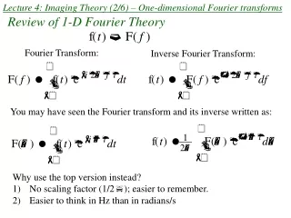
Lecture 4: Imaging Theory (2/6) – One-dimensional Fourier transforms Fourier Transform: Inverse Fourier Transform: Review of 1-D Fourier Theory You may have seen the Fourier transform and its inverse written as: • Why use the top version instead? • No scaling factor (1/2); easier to remember. • Easier to think in Hz than in radians/s
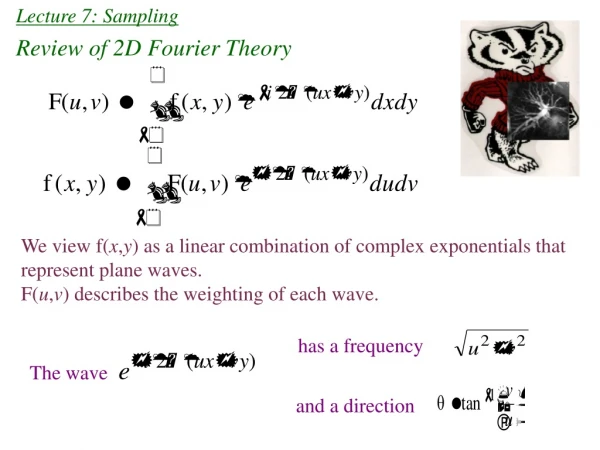
Review of 1-D Fourier Theory, continued Fourier Transform: Let’s generalize so we can consider functions of variables other than time. Inverse Fourier Transform:
Review of 1-D Fourier theory, continued (2) F(u) gives us the magnitude and phase of each of the exponentials that comprise f(x). In fact, the Fourier integral works by sifting out the portion of f(x) that is comprised of the the function exp(+i 2π uox). Orthogonal basis functions f(x) can be viewed as as a linear combination of the complex exponential basis functions.
Some Fourier Transform Pairs and Definitions -1/2 1/2 -1 1
1-D Fourier transform properties If f(x) ↔ F(u) and h(x) ↔ H(u) , Linearity: af(x) + bh(x) ↔ aF(u) + bH(u) Scaling: f(ax) ↔
1-D Fourier transform properties If f(x) ↔ F(u) , Shift: f(x-a) ↔
1-D Fourier transform properties, continued. Say g(x) ↔ G(u). Then, Derivative Theorem: (Emphasizes higher frequencies – high pass filter) Integral Theorem: (Emphasizes lower frequencies – low pass filter)
Even and odd functions and Fourier transforms Any function g(x) can be uniquely decomposed into an even and odd function. e(x) = ½( g(x) + g(-x) ) o(x) = ½( g(x) – g(-x) ) For example, e1 · e2 = even o1 · o2 = even e1 · o1 = odd e1 + e2 = even o1 + o2 = odd
Fourier transforms of even and odd functions Consider the Fourier transforms of even and odd functions. g(x) = e(x) + o(x) Sidebar: E(u) and O(u) can both be complex if e(x) and o(x) are complex. If g(x) is even, then G(u) is even. If g(x) is odd, then G(u) is odd.
Special Cases For a real-valued g(x) ( e(x) , o(x) are both real ), Real part is even in u Imaginary part is odd in u So, G(u) = G*(-u), which is the definition of Hermitian Symmetry: G(u) = G*(-u) (even in magnitude, odd in phase)