Download
1 / 8
80 likes | 229 Vues
Scenario: Kingsthorpe Soil Water Evaporation Project. Justin Fainges APSIM Developer / Mathematician Justin.Fainges@csiro.au. Lead Project Researchers : Jenny Foley - Department of Natural Resources and Mines Jeremy Whish – CSIRO. The Trial.

E N D
Scenario: Kingsthorpe Soil Water Evaporation Project Justin Fainges APSIM Developer / Mathematician Justin.Fainges@csiro.au Lead Project Researchers: • Jenny Foley - Department of Natural Resources and Mines • Jeremy Whish – CSIRO
The Trial Located at Kingsthorpe, QLD. (-27.478, 151.81) Long term evaporation of four soils; a black vertosol, two grey vertisols and a red kandosol. On going, started early 2010. 18 soil monolith weighing lysimeters, 0.6m diameter, 0.8m deep.
The Data Weight changes are measured every 15 minutes. 15 minute data points, 4 reps per soil, 4 soils, 3 years - ~ 1.75 million data points. Daily weights at midnight were analysed. Weather data gathered from on site met station. Very messy due to a number of factors (flood, equipment problems, wildlife, etc). Looking at the Black Vertosol soil from Kingsthorpe. The Task • For the period of April 1 to November 18 2010, use APSIM to model a number of drying curves. • Create a met file using data from an Excel spreadsheet. • Turn the observed data into APSIM format. • Create predicted vs observed plots using the model output.
Daily Weights Very messy in some areas. Noise needs to be accounted for and removed if possible. We will be looking at the highlighted region.
Drying Curves Model 3 periods, 2 April - 4 May, 5 May - 2 July, 11 September – 6 October We will use all the data available and filter it in APSIM.
So How Did We Do? Observed Weights vs. Predicted Weights This graph looks great but is rubbish. Why?
So How Did We Do? Note linearity in deviations. This suggests the error is more in the model parameters than the model itself.