CHAPTER 3 The Church-Turing Thesis

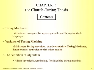
1. CHAPTER 3The Church-Turing Thesis Contents • Turing Machines • definitions, examples, Turing-recognizable and Turing-decidable languages • Variants of Turing Machine • Multi-tape Turing machines, non-deterministic Turing Machines, Enumerators, equivalence with other models • The definition of Algorithm • Hilbert’s problems, terminology for describing Turing machines

2. Variants of Turing Machine (intro) • There are alternative definitions of Turing machines, includingversions with multiple tapes or with non-determinism. • They are called variants of the Turing machine model. • The original model and all its reasonable variants have the same power - they recognize the same class of languages. • In this section we describe some of these variants and the proofs of equivalence in power. Simplest equivalent “generalized” model • In basic definition, the head can move to the left or right after each step: it cannot stay put. • If we allow the head to stay put. The transition function would then have the form • Does this make the model more powerful? Might this feature allow Turing machines to recognize additional languages? • Of course not. We can replace each stay put transition with two transitions, one that moves to the right and the second back to the left.

3. Multi-tape Turing Machine • A multi-tape TM is like an ordinary TM with several tapes. • Each tape has its own head for reading and writing. • Initially the input appears on tape 1, and others are blank. • The transition function is changed to allow for reading, writing, and moving the heads on all tapes simultaneously. Formally, • where k is the number of tapes. • The expression • means that, if the machine is in state q and heads 1 through k are reading symbols trough , the machine goes to state r, writes symbols through , and moves each head to the left or right as specified. … 0 1 0 0 control … a a b b a … b a b • Multi-tape TMs appear to be more powerful than ordinary TMs, but we will show that they are equivalent in power.

4. Multi-tape TMs vs. ordinary TMs • Theorem: Every multi-tape Turing machine has an equivalent single tape Turing • Machine. • We show how to convert a multi-tape TM M to an equivalent single tape TM S. • The key idea is to show how to simulate M with S. • Let M has k tapes. • Then S simulates the effect of k tapes by storing their information on its single tape. • It uses new symbol # as a delimiter to separate the contents of the different tapes. • S must also keep track of the locations of the heads. • It does so by writing a tape symbol with a dot above it to mark the place where the head on that tape would be. • Think of these as ‘virtual’ tapes and heads. … . . . 3 1 S 0 1 M # 0 1 # a a b # b a # … a a b As before, the ‘dotted’ tape symbols are simply new symbols that have been added to the tape alphabet. … b a

5. . . Multi-tape TMs vs. ordinary TMs (cont.) S=“On input • First S puts its tape into the format that represents all k tapes of M. The formatted tape contains • To simulate a single move, S scans its tape from the first #, which marks the left-hand end, to the (k+1)st #, which marks the right-hand end, in order to determine the symbols under the virtual heads. Then S makes a second pass to update the tapes according to the way that M’s transition function dictates. • If at any point S moves one of the virtual heads to the right onto a #, this action signifies that M has moved the corresponding head onto the previously unread blank portion of that tape. So S writes a blank symbol on this tape cell and shifts the tape contents, from this sell until the rightmost #, one unit to the right. Then it continues the simulation as before. . Corollary: A language is Turing-recognizable if and only if some multi-tape Turing machine recognizes it.

6. Non-deterministic Turing Machine • A non-deterministic TM is defined in the expected way: at any point of computation the machine may proceed according to several possibilities. • The transition function for a non-deterministic TM has the form • The computation of a non-deterministic TM N is a tree whose branches correspond to different possibilities for the machine. • Each node of the tree is a configuration of N. The root is the start configuration. • If some branch of the computation leads to the accept state, the machine accepts the input. • We will show that non-determinism does not affect the power of the Turing machine model. • Theorem: Every non-deterministic Turing machine has an equivalent • deterministic Turing Machine. • We show that we can simulate any non-deterministic TM N with a deterministic TM D. • The idea: D will try all possible branches of N’s non-deterministic computation. • The TM D searches the tree for an accepting configuration. If D ever finds an accepting configuration, it accepts. Otherwise, D’s simulation will not terminate.

7. Non-deterministic TMs vs. ordinary TMs • The simulating deterministic TM D has three tapes. By previous theorem this arrangement is equivalent to having a single tape. • Tape 1 always contains the input string and is never altered. • Tape 2 maintains a copy of N’s tape on some branch of its non-deterministic computation. • Tape 3 keeps track of D’s location in N’s non-deterministic computation tree. … 0 1 0 0 Input tape Simulation tape Address tape. D … x x # 0 1 x … 1 2 3 2 3 3 1 • Every node in the tree can have at most b children, where b is the size of the largest set of possible choices given by N’s transition function. • Tape 3 contains a string over Each symbol in the string tells us which choice to make next when simulating a step in one branch in N’s non-deterministic computation. This gives the address of a node in the tree. • Sometimes a symbol may not correspond to any choice if too few choices are available for a configuration. In this case we say that the address is invalid, it does not correspond to any node. • The empty string is the address of the root of the tree.

8. Non-deterministic TMs vs. ordinary TMs (cont.) D=“On input w: • Initially tape 1 contains the input w, and tapes 2 and 3 are empty. • Copy tape 1 to tape 2. • Use tape 2 to simulate N with input w on the branch of its non-deterministic computation. Before each step of N consult the next symbol on tape 3 to determine which choice to make among those allowed by N’s transition function. If no more symbols remain on tape 3 or if this non-deterministic choice is invalid, abort this branch by going to stage 4. Also go to stage 4 if a rejecting configuration is encountered. If an accepting configuration is encountered, accept the input. • Replace the string on tape 3 with the lexicographically next string. Simulate the next branch of N’s computation by going to stage 2.” Corollary 1: A language is Turing-recognizable if and only if some non- deterministic Turing machine recognizes it. In a similar way one can show the following. Corollary 2: A language is Turing-decidable if and only if some non-deterministic Turing machine decides it.

9. Equivalence with other models • We have presented several variants of the Turing Machines and have proved them to be equivalent in power. • Many other models of general purpose computation have been proposed in literature. • Some of these models are very much like Turing machines, while others are quite different (e.g. -calculus). • All share the essential feature of Turing machines, namely, unrestricted access to unlimited memory, distinguishing them from weaker models such us finite automata and pushdown automata. • All models with that feature turn out to be equivalent in power, so long as they satisfy certain reasonable requirements (e.g., the ability to perform only a finite amount of work in a single step). More variants of Turing machine • k-PDA, a PDA with k stacks. • write-once Turing machines. • Turing machines with doubly infinite tape. • Turing machines with left reset • Turing machines with stay put instead of left • If you missed a HW, try to give a complete answer to one of the problems 3.9, 3.11 – 3.14. Only one and complete answer will be accepted. Then you will get 10 points extra credit.