Priority Queues
Priority Queues. Single & Double Ended Priority Q’s. A priority queue is a collection of elements such that each element has an associated priority. SEPQ are categorized as min and max priority queues. SP1: Return an element with minimum priority


Priority Queues
E N D
Presentation Transcript
Priority Queues Single & Double Ended Priority Q’s
A priority queue is a collection of elements such that each element has an associated priority. • SEPQ are categorized as min and max priority queues. • SP1: Return an element with minimum priority • SP2: Insert an element with an arbitrary priority • SP3: Delete an element with minimum priority • The operations supported by max priority queue are same except that in SP1 & SP3 we replace min by max.
[1] [1] 14 2 [2] [2] [3] [3] 12 7 7 4 [4] [4] [5] [5] [6] [6] 10 10 8 8 6 6 • Sample max heaps • sample min heaps
Meldable (single-ended) priority queue, augments the operations SP1 through SP3 with a meld operation that melds together two priority queues. • One applications for the necessary to meld operation is when the server for one priority queue shuts down. It is necessary to meld its priority queue with that of a functioning server.
Double ended priority queue • DP1: Return an element with minimum priority • DP2: Return an element with maximum priority • DP3: Insert an element with an arbitrary priority • DP4: Delete an element with minimum priority • DP5: Delete an element with maximum priority • So, a DEPQ is a min and max priority queue rolled into one structure
Example • Implement a network buffer • Buffer holds packets that are waiting their turn to be sent out over a network link; • Each packet has an associated priority. • When the network link becomes available, a packet with the highest priority is transmitted. This corresponds to a DeleteMax operation. • When a packet arrives at the buffer it is added that corresponds to Insert Operation. • When the buffer is full drop a packet with a min priority that is achieved using a DeleteMin operation.
Leftist Trees • Height-Biased leftist trees • Provide an efficient implementation of meldable priority queues. • Leftist trees are defined using the concept of extended binary tree. • An extended binary tree is a binary tree in which all empty binary subtrees have been replaced by square node. • The square nodes in an EBT are called external nodes and original nodes of BT are called internal nodes.
Extended Binary Trees Example shortest(x): the length of a shortest path from x to an external node.
There are two varieties of leftist-trees • Height Biased (HBLT) • Weight Biased (WBLT) • HBLTs were invented first & are generally referred to simply as leftist trees. • Let x be a node in an EBT. Let leftChild(x) & rightChild(x), denote left & right children of the internal node x. • The shortest(x) satisfies the following recurrence:
Definition • A leftist tree is a binary tree such that if it is not empty, then shortest(leftChild(x)) >= shortest(rightChild(x)) for every internal node x. • Example • Fig. 9.2(a) is not a leftist tree, since shortest(LeftChild(C)=0), whereas shortest(RightChild(C)=1). • Fig. 9.2(b) is a leftist tree.
C delclartions typedefstruct { int key; }element; typedefstruct leftist *leftistTree; struct { leftistTreeleftchild; element data; leftistTreerightchild; intshortext; }leftist;
Min Leftist Tree • A min leftist tree (max leftist tree) is a leftist tree in which the key value in each node is no larger (smaller) than the key values in its children (if any). In other words, a min (max) leftist tree is a leftist tree that is also a min (max) tree.
Example of min leftist trees (b) (a)
Meld Operation…. • We wish to meld the min-leftist trees a & b. • We obtain a new binary tree containing all elements in a & b by following rightmost paths in a & / or b. • This BT has the property that the key in each node is no larger than the keys in its children. • Next we interchange the left & right subtrees of nodes as necessary to convert this BT into a leftist tree.
First compare the root keys 2 & 5 since 2<5 the BT should have 2 in its root. • Leave left subtree of 2 & meld 2’right subtree with entire BT rooted at 5. • when melding the right subtree of 2 & binary rooted 5 notice that 5<50 so 5 should be in the root of melded tree. • No compare 8 & 50 since 8<50 & 8 has no right subtree we can make the subtree with root 50 as right subtree of 8.(fig a) • We begin at the last modified root (ie 8) & check shortest(leftchild())>=shortest(rightchild()). This holds at 8 but not at 5 & 2.
Simply interchange the left & right subtrees and pointer that were interchange are represented by dotted lines in fig. • Function minMeldinterwines two steps. • Create a BT ensure that root of each subtree has the smallest key in that subtree. • Ensure that each node has a left subtree whose shortest value is greater than or equal to that of its right subtree.
Melding the min leftist trees (a) (b)
(c) (d)
Weight-Biased Leftist trees • Definition: A binary tree is a weight-biased leftist tree (WBLT) iff at every internal node the w value of the left child is greater than or equal to the w value of the right child. A max (min) WBLT is max (min) tree that is also a WBLT.
If x is external node, its weight is 0. • If x is an internal node, its weight is 1 more than the sum of the weights of the children.
WBLT Not a WBLT
Binomial Heaps • Cost Amortization • A binomial heap is a data structure that supports the same functions (i.e. insert,delete_min & meld) as those supported by leftist trees. • Let us examine the concept of cost amortization (spread out). • Suppose that a sequence I1,I2,D1,I3,I4,I5,I6,D2,I7 of insert & delete-min operations is performed. • Assume that the actual cost of each of seven inserts in one & delete-min operations have cost of eight & ten respectively
So, the total cost of the sequence of operations is 25. • In a amortization scheme we charge some of the actual cost of an operation to other operations. This reduces the charged cost of an some operations & increases that of others. • The amortized cost of operation is the total cost charged to it. • The cost transferring(amortization) scheme is required to be such that the sum of the amortized costs of the operations is greater than or equal to the sum of their actual costs.
If we charge one unit of the cost of a delete-min operation to each of the inserts then two units of D1 get transferred to I1 & I2 & four units of the cost of D2 get transferred to I3 to I6. • The amortized cost of each of I1 to I6 becomes two, that of I7 is one & that of each D1 & D2 becomes 6. • The sum of amortized costs is 25 which is same as actual costs.
We can prove that no matter what sequence of insert & delete-min operations is performed, we can charge costs in such a way that the amortized cost of each insertion is no more than two & that of each deletion is no more than six. • Using amortization costs we conclude {2i+6d} • Using actual costs we conclude {i+10d} • Combining both {2i+6d,i+10d} as a bound on the sequence cost
8 5 3 15 12 8 10 6 4 20 30 10 Definition of Binomial Heaps • Two varieties of binomial heaps. • Min & max • A min binomial heap is a collection of min trees. • A max binomial heap is a collection of max trees. • Min binomial heaps referred to as B-heaps. 16 16
B-heaps are represented using nodes that have the following fields: • Degree – degree of a node is the number of children it has • Child – child data member is used to point to any one of its children ( if any ) • Link – the link data member is used to maintain single linked circular lists of siblings. • All the children of a node form a singly linked circular list, & node points to one of these children. • Additionally , the roots of the min trees that comprise a B-heap are linked to form a SLCL. • The B-heap is then pointed at by a single pointer min to the min tree root with smallest key.
a) parent c) key degree NIL NIL child sibling 2 1 0 2 head[H] NIL NIL b) 10 12 head[H] 2 1 1 0 NIL NIL 10 12 15 15 0 NIL NIL
Insertion into a Binomial Heap • An element x may be inserted into a B-heap by first putting x into a new node • Then inserting this node into the circular list pointed by min. • The pointer min is reset to this new node only if min is 0 or the key of x is smaller than the key node pointed by min
Melding Two Binomial Heaps • To meld two nonempty B-heaps, we meld the top circular lists of each into a single circular list. • The new B-heap pointer is the min pointer of one of the two trees depending on which has the smaller key. • This can be determined with a single comparision.
Deletion of Min Element • If min is 0, then the B-heap is empty, and a deletion cannot be performed. • Min points to the node that contains min element. • This node is deleted from its circular list. • The new B-heaps consists of the remaining min trees & the sub-min trees of the deleted root.
Before forming the circular list of min tree roots, we join together pairs of min trees that have the same degree. • This min tree joining is done by making the min tree whose root has a larger key a subtree of the other. • When two min trees are joined, the degree of the resulting min tree is one larger than the original degree of each min tree.
Fibonacci Heaps • Two varieties • Min • Max • A min Fibonacci heap is a collection of min trees • A max Fibonacci heap is a collection of max trees • B-heaps are special case of F-heaps • A F-heap is a data structure that supports the three binomial operations: insert,delete min or max & meld as well as • Delete, delete the element in a specified node. (arbitary delete) • Decrease key, decrease the key of a specified node by a given positive amount.
Deletion from an F-heap • To delete an arbitary node b from the F-heap a • If a=b, then do a delete min, otherwise do steps 2,3&4 below. • Delete b from the doubly linked list it is in • Combine the DLL of b’s children with the DLL of a’s min-tree roots to get a SLL. • Dispose of node b.
Decrease Key • To decrease the key in node b • Reduce the key in b. • If b is not a min-tree root & its key is smaller than that in its parent, then delete b from DLL & insert into DLL of min-tree roots. • Change a to point b in case the key in b is smaller than that in a.
Paring Heaps • Experimental results suggest that pairing heaps are actually faster than Fibonacci heaps. • Simpler to implement. • Smaller runtime overheads. • Less space per node. • Defn : A min (max) pairing heap is a min (max) tree in which operations are done in a specified manner.
Pairing heaps come in two varieties – • Min pairing heaps • Max pairing heaps • Min pairing heaps are used when we wish to represent a min priority queue. • Max pairing heaps are used when we wish to represent a max priority queue. • A pairing heap is a single tree, which need not be a binary tree.
9 9 7 7 6 7 6 7 6 3 3 6 Meld & Insert • Compare-Link Operation • Compare roots. • Tree with smaller root becomes leftmost subtree. + = • Actual cost = O(1).
Two min pairing heaps may be melded into a single min pairing heap by performing a compare-link operation. • In compare-link, the roots of the two min trees are compared and the min tree that has the larger root is made the leftmost subtree of the other tree.
9 9 7 6 7 7 6 2 7 3 6 3 6 Insert • Create 1-element max tree with new item and meld with existing max pairing heap. • To insert an element x into a pairing heap p, we first create a pairing heap q with the single element x, & then meld two pairing heaps p & q. = + insert(2)
14 9 9 7 6 7 7 6 7 3 6 3 6 Insert • Create 1-element max tree with new item and meld with existing max pairing heap. = + insert(14) • Actual cost = O(1).
Decrease Key • Suppose we decrease the key/priority of the element in node N. • When N is the root or when the new key in N is greater than or equal to that in its parent, no additional work is to be done. • When the new key is less than that in its parent, the min tree property violated & corrective action to be taken. • The corrective action consists of the following steps • Remove the subtree with root N from the tree. This results in two min trees. • Meld the two min trees together.
Delete Min • The min element is in the root of the tree. So, to delete the min element, we first delete the root node. • When root is deleted, we are left with zero or more min trees. • When the nor of remaining min trees is two or more, these min trees must be melded into a single min tree. • In two pass pairing heaps, this melding is done.
Make a left to right pass over the trees, melding pairs of trees. • Start with the rightmost tree and meld the remaining trees (right to left) into the tree one at a time. • In multi pass pairing heaps, the min trees that remain following the removal of the root are melded into a single min tree as follows. • Put the min trees onto a FIFO queue. • Extract two trees from the front of the queue, meld them & put the resulting tree at the end of the queue. Repeat this step until only one tree remains.
Arbitrary Delete • Deletion from an arbitrary node N is handled as a delete-min operation when N is the root of the pairing heap. When N is not the tree root, the deletion is done as follows. • Detach the subtree with root N from the tree. • Delete Node N & meld its subtrees into a single min tree using the two pass scheme or multi pass scheme. • Meld the min trees from steps 1 & 2 into a single min tree.
9 theNode 6 2 4 6 1 2 1 3 4 5 3 2 3 4 1 Remove theNode from its doubly-linked sibling list.
9 6 2 6 4 1 1 4 5 2 3 2 3 4 3 1 Meld children of theNode.
9 6 2 6 1 1 4 5 3 2 3 4 2 3 1 Meld with what’s left of original tree.
9 6 2 3 6 2 3 1 1 4 5 2 3 4 • Actual cost = O(n). 1