Reactive Empirical Force Fields
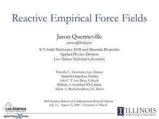
Reactive Empirical Force Fields. Jason Quenneville jasonq@lanl.gov X-1: Solid Mechanics, EOS and Materials Properties Applied Physics Division Los Alamos National Laboratory Timothy C. Germann, Los Alamos Alejandro Strachan, Purdue Adri C. T. van Duin, Caltech

Reactive Empirical Force Fields
E N D
Presentation Transcript
Reactive Empirical Force Fields Jason Quenneville jasonq@lanl.gov X-1: Solid Mechanics, EOS and Materials Properties Applied Physics Division Los Alamos National Laboratory Timothy C. Germann, Los Alamos Alejandro Strachan, Purdue Adri C. T. van Duin, Caltech William A. Goddard III, Caltech Alexei A. Stuchebrukhov, UC Davis 2006 Summer School on Computational Materials Science July 31 - August 11, 2006 · University of Illinois
Motivation Empirical force fields are used in biology, chemistry, physics and materials science to calculate the potential energy surface and atomic forces. Most, like CHARMM and AMBER, assume the same atomic connectivity (molecular composition) throughout simulation. No Chemistry!!! Straightforward solution: ab initio or QM/MM (up to 300 atoms for QM system) For materials simulation, we may want 10s of 1000s to millions of atoms and as much as a nanosecond of simulation time. Need a more efficient method!!!
Empirical Force Fields Empirical force fields contain potential energy functions for each atomic interaction in a molecular system. Bond Stretch: Bond Bending: Bond Torsion: Parameters can be taken from experiment (e.g., vibrational spectroscopy) or from ab initio quantum chemistry calculations.
Empirical Force Fields Non-Bonded potentials give the intermolecular interactions: Coulomb: van der Waals: Parameters obtained through ab initio quantum chemistry and liquid simulations. e.g. OPLS (optimized potentials for liquid simulations, W. L. Jorgensen and J. Tirado-Rives, J. Am. Chem. Soc.110, 1657 (1988). )
Empirical Valence Bond (EVB) EVB attempts to combine empirical potential energy functions with valence bond ideas to describe chemical reactions efficiently and accurately. EVB Applications Proton transport in aqueous acid (CPL, 284, 71 (’98); JPCB, 102, 5547 (’98)) Aqueous acid-base reactions (JPCA, 105, 2814 (‘01)) Enzyme catalysis (Warshel) Nucleophilic substitution reactions Good Introduction: Computer Modeling of Chemical Reactions in Enzymes and Solutions, A. Warshel Wiley-Interscience (02/01/1997)
EVB: introduction EVB starts with a NN potential energy matrix: N diabatic states (diagonal) N(N-1) couplings (off-diagonal) Each diabatic state looks like a configuration in a standard non-reactive force field. Off-diagonal coupling elements: interaction between each diabatic state and the N-1 remaining states. Diagonalize V adiabatic states. The minimal value is the ground state. diabatic states coupling term adiabatic ground state
Calculation of Forces Diagonalizing the NN EVB matrix yields the ground state as a linear combination of diabatic states. If an is the set of corresponding coefficients, the forces can be calculated using the Hellman-Feynman theorem:
EVB: diagonal matrix elements Because we need to treat bond breaking and formation, the Bond Stretch should be anharmonic: Bending and Torsional potentials can be as before: System-environment interactions treated with standard non-bonding potentials:
Interaction between EVB States System-system non-bonding interactions more complicated due to the potential for chemical reaction. A functional form more flexible than Coulomb + Lennard-Jones is required. The intermolecular interactions (part of the diagonal element) and the coupling terms (off-diagonal) must be parametrized together in order to describe the reaction correctly. In the activated complex, the favorable interaction between the two states is controlled by the intermolecular interaction. It is normally written in terms of the distance between the two reactant centers. The reaction barrier is controlled by coupling term. This term is generally a function of the reaction coordinate.
Application: Proton Transfer in Water 0.97 Å 116° 1.2 Å 1.2 Å 118° 118° 0.97 Å 114° 0.97 Å 116° 109° 0.97 Å 0.96 Å 103° 103° 1.22 Å 0.96 Å 1.22 Å 101° Optimized geometries of the {H2O–H–OH2}+ (left) and {HO–H–OH}– (right) complexes, obtained from first principles (MP2/aug-cc-pVTZ).
EVB of H3O+–H2O Proton Transfer Diabatic States: H H H H O H O O H O H H H H Adiabatic State: H H O H O H H
H3O+–H2O Proton Transfer:Coupling Elements H H O H O r H H
EVB vs Ab Initio for H3O+/H2O 2.4 Å 2.6 Å 2.8 Å EVB MP2/aug-cc-pVTZ
EVB Summary Very good for systems with small number of possible reactions Reaction barriers are treated explicitly Offers an empirical description of chemical reactions Gives mixing of diabatic states during reaction Can be difficult to parametrize intermolecular potentials and couplings Limitation on number of states due to diagonalization (cubic scaling)
ReaxFF HN NH N N Bond-Order potential, developed at CalTech by Adri van Duin and Bill Goddard Potential parametrized using ab initio calculations (B3LYP/6-31G**) on a “training set” of reactions Why bond-order based? non-reactive potentials have atom-types that define connectivity Applications: High Explosives, Propellants, Catalysis, Fuel Cells, Corrosion, Friction, etc. + H2
Background References Bond Order/Bond Length relationship Pauling, J. Am. Chem. Soc., 69, 542 (1947). Reactive Empirical Bond Order (REBO) Johnston, Adv. Chem. Phys., 3, 131 (1960). Johnston, Parr, J. Am. Chem. Soc., 85, 2544 (1963). Other Bond-Order Potentials Tersoff, Phys. Rev. Lett., 56, 632 (1986); Tersoff, Phys. Rev. Lett., 61, 2879 (1988). Brenner, Phys. Rev. B, 42, 9458 (1990). Brenner, et al, J. Phys.: Condens. Matter, 14, 783 (2002). ReaxFF van Duin, Dasgupta, Lorant, Goddard, J. Phys. Chem. A, 105, 9396 (2001). Strachan, Kober, van Duin, Oxgaard, Goddard, J. Chem. Phys., 122, 054502 (2005). User Manual: http://www.wag.caltech.edu/home/duin/reax_um.pdf
Charge equilibration: EEM (Mortier, et al, JACS, 108, 4315, (’86).) ReaxFF Potential Energy Function ReaxFF allows for computationally efficient simulation of materials under realistic conditions, i.e. bond breaking and formation with accurate chemical energies. Due to the chemistry, ReaxFF has a complicated potential energy function:
Bond Order, Bond Energy Example: Acetylene Bond Order goes smoothly from 0 1 2 3 as C-C Bond Length shortens from large distance to 1.0 Å Bond Order C-C Distance / Å …not explicitly a function of bond distance
Bond Order Corrections Bond orders adjusted to get rid of unphysical bonds. Over- and under-coordination of atoms must be avoided. Energy penalty added to the potential energy function for the case where an atom has more bonds than its valence allows. e.g., Carbon can’t have more than 4 bonds; Hydrogen no more than 1 If an atom is under-coordinated, the stabilization of p bonding should be used if possible.
Bond Angles, Bond Torsion Bond Angles and Torsions are intimately tied to the bond types. With a bond order potential, angles and torsions must be written in terms of the bond order. Angle and torsion energy terms must 0 as B.O. 0. CCH 120° CCH = 180° See J. Phys. Chem. A, 105, 9396 (2001) for full potential form.
Lone Pair Electrons, Conjugation implicit in AMBER/CHARMM-like potentials through atom type The creation or reaction of lone-pair electrons should be assigned an energy term. Elone pair corresponds to an energy penalty for having too many lone pairs on an atom (i.e., overcoordination) Conjugated systems should have added stabilization. Econj has maximum contribution when successive bonds have bond-order values of 1.5.
Hydrogen Bonding Hydrogen bonding extremely important in biological systems but also in many organic solids. X – H Y Hydrogen bonds are calculated between group X-H and Y, where X and Y are atoms known to form H-bonds (e.g., N, O) The H-bond energy term is written in terms of the bond-order of X-H, the distance between H and Y, as well as the X-H-Y angle. Can be an expensive part of the calculation because many acceptor (Y) atoms could be available for any given X-H group. All interactions must be calculated out to a cutoff distance (~10 Å) in order to remain consistent from timestep to timestep.
Non-Bonded Interactions - Short-range Pauli Repulsion - Long-range attraction (dispersion) - Coulomb forces van der Waals and Coulomb terms are includedfor all atom pairs (whether bonded or non-bonded)! This avoids changing the potential when chemistry occurs. Such alterations, which are natural in the EVB formalism, would be awkward in ReaxFF. Shielding included for both Coulomb and van der Waals in order to avoid excessive interaction between atoms sharing bond and/or bond angle. Energy / kcal mol-1 Interatomic Distance / Å
Charge Equilibration HN NH N N The charge on an atom depends on the molecular species: Atomic charges are adjusted with respect to connectivity and geometry. Many QEq methods available. ReaxFF uses Electronegativity Equalization Method (EEM: Mortier, et al, JACS, 108, 4315, (’86).) The desired charge distribution is that which minimizes, Final Coulomb energy from screened potential – all atom-pairs calculated + H2
ReaxFF/Ab Initio Comparison ReaxFF can decribe a wide variety of chemical reactions. e.g., unimolecular decomposition of RDX Strachan, et al, JCP, 122, 054502 (’05).
Application: HE at High T, P 768 atoms (32 molecules, 224 unit cells) • Interested in chemical reaction dynamics of high explosives (HE) under shock conditions • Want as big a system (105 to 106 atoms) as possible in order to study the spread of reactions, temperature distribution, carbon-clustering, etc. TATB 103,680 atoms (4320 molecules, 121215 unit cells) 256 processors
Decomposition of TATB at High T CO2 Tinitial = 1700 K Tfinal = ~3200 K H2O N2 TATB
ReaxFF in Parallel • GRASP (General Reactive Atomistic Simulation Program) developed at Sandia National Lab by Aidan P. Thompson. • Objective: Parallel scalable MD code (C++) which enables implementation of a wide range of force field types, particularly reactive force fields, including ReaxFF. CPU Time per timestep: serial code: 2.8 seconds parallel code: 0.6 seconds (32 CPUs) System size limits: serial code: 5000 atoms parallel code: 500,000 atoms (510 CPUs) ASC Flash: 2.0-GHz procs 8 GB memory per node
ReaxFF Summary Time/Iteration (seconds) Natoms Can simulate chemistry for a wide range of materials significantly faster than ab initio and semi-empirical methods Accuracy similar to semi-empirical methods Hydrocarbons, CHNO explosives, silicon oxides, etc. Main limitation is governed by the size of reaction training set Used extensively for explosives under extreme conditions - many possible reactions Simulation sizes up to a half million atoms