FAUST Technology for Classifiers: Fast, Analytic, Unsupervised, and Supervised
150 likes | 173 Vues
Utilize the innovative FAUST technology for fast and accurate classification, incorporating both unsupervised and supervised methods. The FAUST system includes One-Class Spherical (OCS), One-Class Linear (OCL), and Multi-Class Linear (MCL) classifiers for effective data analysis. Benefit from the ability to construct enclosures, hulls, and spheres to classify samples accordingly. Explore the comprehensive FAUST classification system for enhanced efficiency in data processing and pattern recognition.

FAUST Technology for Classifiers: Fast, Analytic, Unsupervised, and Supervised
E N D
Presentation Transcript
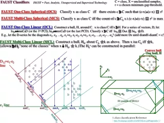
Oblique FAUST ClassifiersFast, Analytic, Unsupervised and Supervised Technology C = class, X = unclassified samples, r a chosen gap threshold. FAUST One-Class Spherical (OCS)Construct a sphere, around x. x isa C iff the sphere hits C. Classify x into C iff there exists cC such that (c-x)o(c-x) r2 a a a a a a a a aa a a a a aa a c c c c c c c c cc c c c c cc c b b b b b b b b bb b b b b bb b D=e1+e2+e3 D=e1-e3 e3 e2 D=e1+e3 e1 mxBoD12 mxCoD12 mxAoD12 mnB1 mxA1 mxB1 mnA1 mnC1 mxC1 mnBoD12 mnCoD12 mnAoD12 FAUST One-Class Linear (OCL)Construct a tight enclosure, a hull, H, around C. x isa C iff xH. D in a series, loDmnCoD (or 1st PCI); hiDmxCoD (or last PCD). Classify xC iff loD Dox hiD D. D-series = diagonals e1, e2, ...en, e1+e2, e1-e2, e1+e3, e1-e3, ...,e1-e2-...-en? (add Ds until diamH - diamC < ε ? FAUST Multi-Class Linear (MCL)Construct non-intersecting hull, Hk, Ck. then x isa Ck iff xHk. Classify x isa Ck iff lok,D Dox hik,D D. FAUST MCL allows for a "none of the classes" when xHk, k. In FAUST MCL the Hks can be constructed in parallel: Convex hull Our hull, H c c c c c c c c cc c c c c cc c D12=e1-e2 line 3D example of HULL1 e1 line 1-class classification Reference : http://homepage.tudelft.nl/n9d04/thesis.pdf#appendix*.7
FAUST OCS One Class Spherical classifier to the Spaeth dataset as a "lazy" classifier Let the Class be {yb,yc.yd,ye}. 1class classify unclassified sample, yf. Let r=3. So yf is not in C since it is spherically gapped away from C by r=3 units. How expensive is the algorithm? For each x 1. Compute the SPTS, ESDx as (C-x)o(C-x) 2. Compute the mask pTree, ESDx < r2 3. Count i-bits in that mask pTree. C1 pTrees C2 pTrees C C1 13 12 11 10 C2 23 22 21 20 ESDx yb 10 1 0 1 0 9 1 0 0 1 10 yc 11 1 0 1 1 10 1 0 1 0 20 yd 9 1 0 0 1 11 1 0 1 1 13 ye 11 1 0 1 1 11 1 0 1 1 25 yf 7 0 1 1 1 8 1 0 0 0 0 1 y1y2 y7 2 y3 y5 y8 3 y4 y6 y9 4 ya 5 6 7 8 yf 9 yb a yc b yd ye 0 1 2 3 4 5 6 7 8 9 a b c d e f Shortcut for 1.d,e,f by some comparison of hi bitslices of ESD with #9? (I think Yue Cui has a shortcut here???) C1 13 12 11 10 C2 23 22 21 20 yb 10 1 0 1 0 9 1 0 0 1 yc 11 1 0 1 1 10 1 0 1 0 yd 9 1 0 0 1 11 1 0 1 1 ye 11 1 0 1 1 11 1 0 1 1 x=yf 7 0 1 1 1 8 1 0 0 0 1a Compute SPTS (C-x)o(C-x): Shortcut for 1.a,b,c,d,e,f: (C-x)o(C-x) = CoC -2Cox +|x|2 < r2 C as a PTS is: and x=yf is: |x|2-r2 + CoC < 2Cox 1.b Form cosntant SPTSs #7 3 2 1 0 #8 3 2 1 0 #9 3 2 1 0 7 0 1 1 1 8 1 0 0 0 9 1 0 0 1 7 0 1 1 1 8 1 0 0 0 9 1 0 0 1 7 0 1 1 1 8 1 0 0 0 9 1 0 0 1 7 0 1 1 1 8 1 0 0 0 9 1 0 0 1 1.c Construct (C-x)o(C-x) by SPTS arithmetic: ESD=(C1-#7)(C1-#7) + (C2-#8)(C2-#8) (faster way?) 4 3 2 1 0 10 0 1 0 1 0 20 1 0 1 0 0 13 0 1 1 0 1 25 1 1 0 0 1 Precompute (1 time) SPTS CoC and PTS 2C (2C is just a relabeling of pTrees of C). For each new unclassified sample, x, add |x|2-r2 to CoC (adding one constant to one SPTS) compute 2Cox (n multiplications of one SPTS, 2Ci, by one constant, xi' then add the n resulting SPTSs. compare |x|2-r2 +CoC to 2Cox giving us a mask pTree count 1-bits in this mask pTree (shortcuts?, shortcuts?, shortcuts?) 1.d Construct the mask pTree (C-x)o(C-x) < #9 (How?) 0 0 0 0 1.e Count the 1 bits = 0 1.f Conclude that yfC This is no longer a lazy classifier, but a model-based classifier, since we're building a model by precomputing CoC and 2C
FAUST OCS One Class Spherical classifier to the Spaeth dataset as a model-based classifier Let the Class be {yb,yc.yd,ye}. 1class classify unclassified sample, yf. Let r=3. 1 y1y2 y7 2 y3 y5 y8 3 y4 y6 y9 4 ya 5 6 7 8 yf 9 yb a yc b yd ye 0 1 2 3 4 5 6 7 8 9 a b c d e f 1. Precompute CoC, 2C=shift-left-1 of C. For each new unclassified sample, x, 2. add a = |x|2-r2 to CoC 3. compute 2Cox 4. a +CoC < 2Cox 5. count 1-bits in this mask pTree C1 pTrees C2 pTrees C C1 13 12 11 10 C2 23 22 21 20 yb 10 1 0 1 0 9 1 0 0 1 yc 11 1 0 1 1 10 1 0 1 0 yd 9 1 0 0 1 11 1 0 1 1 ye 11 1 0 1 1 11 1 0 1 1 yf 7 0 1 1 1 8 1 0 0 0 CoC pTrees CoC 7 6 5 4 3 2 1 0 181 1 0 1 1 0 1 0 1 221 1 1 0 1 1 1 0 1 202 1 1 0 0 1 0 1 0 242 1 1 1 1 0 0 1 0 2C1 pTrees 2C2 pTrees 2C1 14 13 12 11 2C2 24 23 22 21 20 1 0 1 0 18 1 0 0 1 22 1 0 1 1 20 1 0 1 0 18 1 0 0 1 22 1 0 1 1 22 1 0 1 1 22 1 0 1 1 a = |x|2-r2 = 104 CoC+a pTrees CoC+a 8 7 6 5 4 3 2 1 0 285 1 0 0 0 1 1 1 0 1 325 1 0 1 0 0 0 1 0 1 306 1 0 0 1 1 0 0 1 0 346 1 0 1 0 1 1 0 1 0 2Cox pTrees 2Cox 8 7 6 5 4 3 2 1 0 284 1 0 0 0 1 1 1 0 0 314 1 0 0 1 1 1 0 1 0 302 1 0 0 1 0 1 1 1 0 330 1 0 1 0 0 1 0 1 0 CoC+a>2Cox 0 0 0 0 Ct=0 so x not in C Shortcuts to 1? Yes, 2C is just a renaming of pTrees and even tho CoC is a 1-time precomputations, a shortcut would help. Shortcuts to 2? Yes, just use the bit pattern of a. Shortcuts to 3? Possibly just use the bit patterns of x1 and x2? Shortcuts to 4? In 2's Complement, subtract and look at the sign bit??? Shortcuts to 5? Shortcuts that combine any or all of these?
FAUST OCS One Class Spherical classifier to the Spaeth dataset as a model-based classifier Let the Class be {yb,yc.yd,ye}. 1class classify unclassified sample, x=(a,9). Let r=3. 1 y1y2 y7 2 y3 y5 y8 3 y4 y6 y9 4 ya 5 6 7 8 yf 9 yb a yc b yd ye 0 1 2 3 4 5 6 7 8 9 a b c d e f 1. Precompute CoC, 2C=shift-left-1 of C. For each new unclassified sample, x, 2. add a = |x|2-r2 to CoC 3. compute 2Cox 4. a +CoC < 2Cox 5. count 1-bits in this mask pTree C1 pTrees C2 pTrees C C1 13 12 11 10 C2 23 22 21 20 yb 10 1 0 1 0 9 1 0 0 1 yc 11 1 0 1 1 10 1 0 1 0 yd 9 1 0 0 1 11 1 0 1 1 ye 11 1 0 1 1 11 1 0 1 1 x 10 0 1 1 1 9 1 0 0 1 x CoC pTrees CoC 7 6 5 4 3 2 1 0 181 1 0 1 1 0 1 0 1 221 1 1 0 1 1 1 0 1 202 1 1 0 0 1 0 1 0 242 1 1 1 1 0 0 1 0 2C1 pTrees 2C2 pTrees 2C1 14 13 12 11 2C2 24 23 22 21 20 1 0 1 0 18 1 0 0 1 22 1 0 1 1 20 1 0 1 0 18 1 0 0 1 22 1 0 1 1 22 1 0 1 1 22 1 0 1 1 a = |x|2-r2 = 172 CoC+a pTrees CoC+a 9 8 7 6 5 4 3 2 1 0 724 1 0 1 1 0 1 0 1 0 0 884 1 1 0 1 1 1 0 1 0 0 808 1 1 0 0 1 0 1 0 0 0 968 1 1 1 1 0 0 1 0 0 0 2Cox pTrees 2Cox 8 7 6 5 4 3 2 1 0 362 1 0 1 1 0 1 0 1 0 400 1 1 0 0 1 0 0 0 0 378 1 0 1 1 1 1 0 1 0 418 1 1 0 1 0 0 0 1 0 CoC+a>2Cox 1 1 1 1 Ct=4 so x in C Shortcuts to 5? There should be a primitive "pTree not pure zero" which returns 1 or 0. The micro code might simply apply a table look up over and over but only until the first lookup is nonzero. I think Dr. Wettstein has such a primitive. Shortcuts to 4+5? Compare from high order bit side until first indication that a row comparison is <
For WINE with C=class4 and outliers=class7 (Class 4 was enhanced with 3 class3's to fill out the 50) For CONCRETE, concLH with C=class(8-40) and outliers=class(43-67) The 1D model classifies 50 class1 and 43 class3 incorrectly as class1. The 1D model classifies 50 class1 and 48 class3 incorrectly as class1. For SEEDS with C=class1 and outliers=class2 For IRIS with C=Vers, outliers=Virg,FAUST 1D: SLcutpts (49,70); SWcutpts(22,32); PLcutpts(33,49); PW Ctpts(10,16) 44 vers correct. 7 virg errors The 1D model classifies 50 class1 and 15 class2 incorrectly as class1. The 1D_2D model classifies 50 class1 and 43 class3 incorrectly as class1. The 1D_2D model classifies 50 class1 and 35 class3 incorrectly as class1. Trim outliers: 20;34 30:50,51 18 The 1D_2D model classifies 50 class1 and 8 class2 incorrectly as class1. The 1D_2D_3D model classifies 50 class1 and 30 class3 incorrectly as class1. The 1D_2D_3D model classifies 50 class1 and 43 class3 incorrectly as class1. The 1D_2D_3D model classifies 50 class1 and 8 class2 incorrectly as class1. 1D_2D model classifies 50 vers (no eliminated outliers) and 3 virg in the 1class The 1D_2D_3D_4D model classifies 50 class1 and 27 class3 incorrectly as class1. The 1D_2D_3D_4D model classifies 50 class1 and 42 class3 incorrectly as class1. The 1D_2D_3D_4D model classifies 50 class1 and 8 class2 incorrectly as class1. 1D_2D_3D model classifies 50 vers (no eliminated outliers) and 3 virg in the 1class For CONCRETE, concM (class is the middle range of strengths) The 1D model classifies 50 class1 and 47 class3 incorrectly as class1. 1D_2D_3D_4D model classifies 50 vers (no eliminated outliers) and 3 virg in the 1class For SEEDS with C=class1 and outliers=class3 The 1D_2D model classifies 50 class1 and 37 class3 incorrectly as class1. The 1D model classifies 50 class1 and 30 class3 incorrectly as class1. The 1D_2D_3D model classifies 50 class1 and 30 class3 incorrectly as class1. The 1D_2D model classifies 50 class1 and 27 class3 incorrectly as class1. The 1D_2D_3D model classifies 50 class1 and 27 class3 incorrectly as class1. The 1D_2D_3D_4D model classifies 50 class1 and 26 class3 incorrectly as class1. The 1D_2D_3D_4D model classifies 50 class1 and 27 class3 incorrectly as class1. For SEEDS with C=class2 and outliers=class3 The 1D model classifies 50 class1 and 0 class3 incorrectly as class1. The 1D_2D model classifies 50 class1 and 0 class3 incorrectly as class1. The 1D_2D_3D model classifies 50 class1 and 0 class3 incorrectly as class1. The 1D_2D_3D_4D model classifies 50 class1 and 0 class3 incorrectly as class1. FAUST OCL One Class Linearclassifier applied to IRIS, SEEDS, WINE, CONCRETE datasets For series of D's = diagonals e1, e2, ...en, e1+e2, e1-e2, e1+e3, e1-e3, ...,e1-e2-...-en The 3 persistent virg errors virg24 63 27 49 18 virg27 62 28 48 18 virg28 61 30 49 18
Class1=C1={y1,y2.y3,y4. FAUST MCL Multi-Class Linear classifier of the Spaeth dataset Class2=C2={y7,y8.y9}. C e1 13 12 11 10 e2 23 22 21 20 y1 1 0 0 0 1 1 0 0 0 1 y2 3 0 0 1 1 1 0 0 0 1 y3 2 0 0 1 0 2 0 0 1 0 y4 3 0 0 1 1 3 0 0 1 1 y7 15 1 1 1 1 1 0 0 0 1 y8 14 1 1 1 0 2 0 0 1 0 y9 15 1 1 1 1 3 0 0 1 1 yb 10 1 0 1 0 9 1 0 0 1 yc 11 1 0 1 1 10 1 0 1 0 yd 9 1 0 0 1 11 1 0 1 1 ye 11 1 0 1 1 11 1 0 1 1 mn1 1 mx1 3 mn2 1 mx2 3 mn1+2 2 mx1+2 6 mn1-2 0 mx1-2 2 mn1 14 mx1 15 mn2 1 mx2 3 mn1+2 16 mx1+2 18 mn1-2 12 mx1-2 14 mn1 9 mx1 11 mn2 9 mx2 11 mn1+2 20 mx1+2 22 mn1-2 -1 mx1-2 1 Class3=C3={yb,yc.yd,ye} 1 y1y2y7 2 y3y5 y8 y 3 y4 y6 y9 4 ya 5 6 7 8 yf 9 yb ax yc b yd ye 0 1 2 3 4 5 6 7 8 9 a b c d e f Classify xCk iff lok,D Dox hik,D D. xf 7 Just on the basis of e1 it is "none-or-the-above" 9,a 9 -1 19 10 It is in class3 (red) only ya 13 Just on the basis of e1 it is "none-or-the-above" y5 5 2 Just on the basis of e1 it is "none-or-the-above" f,2 15 13 17 2 It is in class2 (green) only Shortcuts for MCL? Precompute all diagonal minimums and maximums; e1, e2, e1+e2, e1-e2. Then,,in fact, there is no pTree processing left to do (just straight forward number comparisons).
FAUST MCL Multi-Class Linear classifier of IRIS dataset Classify xCk iff lok,D Dox hik,D D. Versicolor 1D min 49 20 33 10 max 70 34 51 18 n1 n2 n3 n4 x1 x2 x3 x4 1D MCL Hversicolor has 7 virginica! Versicolor 2D min 70 82 59 55 59 43 24 9 38 -24 7 23 max 102 118 84 80 84 67 40 23 56 -7 18 35 n12 n13 n14 n23 n24 n34 n1-2 n1-3 n1-4 n2-3 n2-4 n3-4 x12 x13 x14 x23 x24 x34 x1-2 x1-3 x1-4 x2-3 x2-4 x3-4 1D_2D MCL Hversicolor has 3 virginica! Versicolor 3D min 105 80 92 65 35 58 -21 60 35 max 149 116 134 98 55 88 -2 88 55 n123 n124 n134 n234 n12-3 n1-23 n1-2-3 n12-4 n1-24 x123 x124 x134 x234 x12-3 x1-23 x1-2-3 x12-4 x1-24 9 72 24 -7 45 -9 -40 28 103 37 12 65 6 -19 n1-2-4 n13-4 n1-34 n1-3-4 n23-4 n2-34 n2-3-4 x1-2-4 x13-4 x1-34 x1-3-4 x23-4 x2-34 x2-3-4 1D_2D_3D MCL Hversicolor has 3 virginica! Versicolor 4D min 115 95 45 68 20 48 -6 -39 max 164 135 69 104 41 74 10 -12 n1234 n123-4 n12-34 n1-234 n12-3-4 n1-23-4 n1-2-34 n1-2-3-4 x1234 x123-4 x12-34 x1-234 x12-3-4 x1-23-4 x1-2-34 x1-2-3-4 1D_2D_3D_4D MCL Hversicolor has 3 virginica (24,27,28) 1D_2D_3D_4D MCL Hvirginica has 20 versicolor errors!! Why? Next slide I look at removing outliers from the Hullvirginica
FAUST MCL Multi-Class Linear classifier on IRIS Create Hullviriginica with outliers removed (if gap 3) before setting cut points. W/o outlier removal, 1D_2D_3D_4D MCL Hvirginica has 20 versicolor errors!! e1 Ct gp 49 1 7 56 1 1 57 1 1 58 3 1 59 1 1 60 2 1 61 2 1 62 2 1 63 6 1 64 5 1 65 4 2 67 5 1 68 2 1 69 3 2 71 1 1 72 3 1 73 1 1 74 1 2 76 1 1 77 4 2 79 1 e2 Ct gp 22 1 3 25 4 1 26 2 1 27 4 1 28 8 1 29 2 1 30 12 1 31 4 1 32 5 1 33 3 1 34 2 2 36 1 2 38 2 e3 Ct gp 18 1 27 45 1 3 48 1 1 49 3 1 50 3 1 51 7 1 52 2 1 53 2 1 54 2 1 55 3 1 56 6 1 57 3 1 58 3 1 59 2 1 60 2 1 61 3 2 63 1 1 64 1 2 66 1 1 67 2 2 69 1 e4 Ct gp 14 1 1 15 2 1 16 1 1 17 1 1 18 11 1 19 5 1 20 6 1 21 6 1 22 3 1 23 8 1 24 3 1 25 3 12 Ct gp 74 1 8 82 2 2 84 1 1 85 2 1 86 1 1 87 1 1 88 1 1 89 1 1 90 3 1 91 3 1 92 4 3 95 4 1 96 3 1 97 3 1 98 2 2 100 5 1 101 2 1 102 3 1 103 1 1 104 1 1 105 1 1 106 1 1 107 1 1 108 1 7 115 1 2 117 1 13 Ct gp 78 1 16 94 1 10 104 ... 146 14 Ct gp 66 1 9 75 2 1 ... 102 1 23 Ct gp 48 1 22 70 1 2 72 1 3 75 2 1 ''' 96 1 1 97 1 5 102 1 3 105 1 24 Ct gp no outliers 34 Ct gp 36 1 26 62 1 3 65 1 1 ... 89 1 3 92 1 Hvirginica w ouliers removed 15 versic Hvirginica w ouliers removed 3 versic Hvirginica w ouliers removed 12 versic 1D MCL Hvirginica w these 3 ouliers removed, has only 16 versicolors! So we can get it down from 20 to 3 versicolor errors in Hvirginica but by throwing out 15 outlier virginica? Should we do that? It is true that the 15 virginica we throw out of Hvirginica are far away from the others but they are virginica and they are not in Hversicolor for the most part???? One possibility would be to keep track of those (that are outliers to their class but are not in any other class hull and put a sphere around them. Then any unclassified sample that doesn't fall in any class hull would be checked to see if it falls in any of the class outlier spheres???
THESIS ARIJIT I have signed up for a membership under http://www.eoddata.com/ from where I have downloaded historical data. There are variety of indexes whose data has been shared but most popular one to look at will be NASDAQ. There is a dataset which provides you with detailed information for each stocks traded under NASDAQ on a particular day. I have attached this for your reference. This contains all the data for all the stocks which have been traded for last 7 days. We can also find the detailed behavior of each of these stocks as well in an interval of 1 min, 5 minute, 15 minute, 60 mins and so on. I am also not looking for coming up with a new prediction model but how we can necessarily cluster similar nature stocks together. So that when am studying the behavior of stock X I know that the behavior of stock Y might be related as they have reacted to similar market behaviors earlier. Right now, in my pen and paper model what I do is I look at the charts very thoroughly from a span of 5 days, 1 month , 3 months and try to understand the valuation of the stock on that particular day whether its worth or not. I also am studying the stock tweets and market news and am trying to gather whether the general consensus on that stock is positive or negative. I am not too concerned on every minute tradings ( so here PTree will play in as we can reload the memory with the historical data already and will need to include the data only from the last trading day into the memory each time we process). So here the things I mine are: current market news ( text mining), then studying tweets ( by variety of people), then most important the charts. I put emphasize on quarterly reports and feel that the timing is the key above all. "When to buy" and "When to Sell" would be the biggest questions. Historically a stocks valuation gets affected during the quarterly time frame. In this quarter Hope this gives you an idea how am doing the analysis and where we can fit our technology in this space. I think there is a potential opportunity for all of us. I just want to come up with looking at this aspect as have not seen many articles or research papers around this area. Feel free to pass me along if you stumble upon something which you might feel interesting. I was also lucky enough to see Bill Gates, Steve Ballmer and Satya Nadella the other day on campus. WP Reply: Along these lines, please give some thought to the following idea: Yes, there are billions of dollars and millions of people focusing on data mining algorithms to crack the stock market. And, yes, that would seem to make it unlikely that you and I can come up with anything new – EXCEPT THAT: We have an entirely different approach (as confirmed by Mark Silverman at Treeminer and his US government clients and confirmed actually by Mike Stonebreaker when Len Shapiro presented the pTree ideas to him). So…. Is there a dataset out there that is just too deep (too many records) for our competition to process and therefore one that has potential critical info in it but scares people away because of its massive cardinality? If we can find that one and use FAUST on it, done!
Opening Bell Opportunity Evaluator (OBOE): The NYSE Bell is at 9AM EST (I think). At 8:53AM EST (EST=UTC-5), create Trends Around the Globe (TAG) pTrees(1 if the stock is on an upswing, 0 if it is on a downswing) for the London Stock Exchange (2PM UTC), Paris (3PM UTC+1), Frankfurt (3PM UTC+1), as well as Closing Trends at Tokyo, Shanghai, Korean, Bombay, Singapore, … Each of these pTrees would use the same ordered list of rows (same stocks in alphabetical order, so, e.g., the 5th bit is Microsoft in all cases, etc.). OBOE would recommend BUY iff the AND of all TAGs is 1. Actually this is probably being done since the TAGs are small data. What would be big data of the same genre that noone would think of tackling due to the immense size??
THESES: Mohammad and Arjun are approaching the deadline for finishing and since they are working in related areas, I thought I would try to lay out my understanding of what your theses will be (to start the discussion). Mohammad’s thesis might be titled something like, “Horizontal Operators and Operations for Mining Big Vertical Data” and could detail and compare the performance of all the PTS operators we use and the various implementation methods. Keep in mind, that “best” may vary depending upon lots of things, such as the type of data, the type of data mining, the size of the data, the complexity of the data, etc. Even though I often recommend paper type thesis, It seems that non-paper theses are more valuable (witness how many times I refer to Yue Cui’s) Arjun’s thesis could be titled “Performance Evaluation of the FAUST Methodology for Classification, Prediction and Clustering” and will compare the performance of all data mining methods in the FAUST genre (to the others in the FAUST genre and at least roughly to the other main methods out there). The point should be made up front that for big vertical data, there aren’t many implementations and the issue is speed because applying traditional methods (to the corresponding horizontal version of the data) takes much too long. The comparison to traditional horizontal data methods can be explained to be limited to showing that pTree methods compare favorably to those others on accuracy, and with respect to speed, the comparison can be a rough Big-O comparison (and might also bring in the things Dr. Wettstein pointed out to us (see the 1_4_14 notes). Of course give reference if you do. The structure chart for FAUST might be: Then any of these modules might call any or all Mohammad’s SPTS procedures and some of my stuff as well as Dr. Wettstein’s procedures These procedures include: Dot product add/subtr/mult/mult_by_constant SPTSs. My thinking was that you would performance analyze the structure chart stuff above and Mohammad would detail his 2’s comp stuff and then performance analyze it (and various implementations of his stuff) as well as the other lower level procedural stuff.Both of you would consider the various dataset types and sizes and both would quote the results of the other probably FAUST ARM? Classification (Cut-pt where? Clustering Outlier detection 1 class Classification gapped singleton cluster lazy NN= Md's thesis will detail (essentially on SPTS Operations) Computing Squared Euclidean Distance, SED, from a point, p: (Yop)2, Y is a set and p is a fixed pt in n-space Yop = i=1..n(yipi) ED(y,p) = SQRT(i=1..n(yi – pi)2 ) SED(y,p) = i=1..n(yi – pi)2 = i=1..n(Yi-pi)(Yi-pi) = i=1..n(YiYi – 2piYi + pi2 ) = i=1..nYiYi – 2i=1..npiY + pop Md: I can calculate (Yi-pi) using 2's complement then multiply (Yi-pi) with (Yi-pi) to get the (Yi-pi)2, then add them for i=1..n giving SED (Squared Euclidian Distance). But if we break up: i=1..n(Yi-pi)2 = i=1..n(Yi2 - 2Yipi + pi2) = i=1..nYi2 - 2i=1..nYipi + i=1..npi2 I think we need more multiplication than addition which is an expensive operation. I have a little example comparing these two methods. D-line sequence Cut-pt where? mean-midpt VOM-midpt means-STD-ratio medians-STD-ratio Mean-VoM Cycle_diags Mean-furthest gap count_change others Lazy Model Model-high-value (diagonal planes) round-corners barrel sphere
Oblique FAUST CC: Cuts are made at count changes, not just at gaps. Count changes reveal the entry or exit of a cluster by the perpendicular hyper-plane. This improves Oblique FAUST's ability to cluster big data (compared to cutting only at gaps.). We tried Oblique FAUST CC on Spaeth dataset successfully (produces a full dendogram of sub-clusterings by recursively taking the dot product with the vector from the Mean to the VOM (Vector-Of-Medians) and by cutting at each 25% count change in the interval count distribution produced by the UDR procedure with interval widths of 23 . We claim that an appropriate count change will reveal cluster boundaries almost always. i.e., almost always a precipitous count decrease will occur as the cut hyper-plane enters a cluster and a precipitous count increase will occur as the cut hyper-plane exits a cluster. We also claim that Improved Oblique FAUST will scale up for big data, because entering and leaving clusters "smoothly" (without noticeable count change) is no more likely for big data than for small. (since it's a measure=0 phenomenon). For the count changes to reveal themselves, it may be necessary in some data settings to look for a change pattern over a distribution window because entering a round cluster may not produce a large abrupt change in counts but may produce a noticeable change pattern over a window of counts. It may be sufficient for this purpose to just use a naive windowing in which we stop the UDR count distribution generation process at intervals of width=2k for some small value of k and look for consecutive count changes in that rough count distribution. This approach appears to be effective and is fast. We built the distribution down to intervals of width 23=8 for the Spaeth dataset, which has diameter=114. So, for Spaeth we stopped UDR at interval widths equal to 7% of the overall diameter (8/114=.07). Outliers, especially exterior outliers, can produce a bad diameter estimate. To get a good cluster diameter estimate, we should identify and mask off exterior outliers first (before applying the Pythagorean diameter estimation formula). Cluster outliers can be identified as singleton sub-clusters that are sufficiently gapped away from the rest of the cluster. Note that pure outlier or anomaly detection procedure need not use the Improved Oblique FAUST method since outliers are always surrounded by gaps and they do not produce big count changes. Pts furthest from [or just far from] VOM are high probability candidates for exterior outliers. These can be identified and then checked for outliers by creating SPTS, (YoVOM)2 and use just the high end of the UDR to mask those candidates. Of course points that project at the extremes of any dot product projection set are outlier candidates too. FAUST Technology for Clustering and Classification is built for speed improvements so that big data can be mined in human time. Improved Oblique FAUST places cuts at all large Count Changes, each of which reveals a cluster boundary almost always (i.e., almost always a large count decrease occurs iff we are exiting a cluster on the cut hyper-plane and a large count increase occurs iff we are entering a cluster. IO FAUST makes a cut at each large count change in the yod values (A gap is a large decr followed by a large incr, so gaps are included) & is Divisive Hierarchical Clustering IO FAUST scales up (entering and leaving a cluster "smoothly" is a measure=0 phenomenon). Works just as well for big data. A radius estimate for a set, Y, is SQRT( (width(Yod)/2)2 + (max d-barrel radius)2 ), assume all outer edge outliers removed Density Uniformity(DU) of a sub-cluster defined as the reciprocal of the variance of the counts. dendogram has a Density=count/volume label and a Density Uniformity=reciprocal_of_count_variance label on each edge. We can end a dendogram branch as soon as Density and Density Uniformity are high enough (> thresholds, DT and DUT) to save time. We can [quickly] estimate Density as count/cnrn. We have the count a radius estimate and n. cn is a known constant (e.g., c1=, c2=4/3...).. Decide on a density threshold, DET, and a Density Uniformity Threshold DUT. To choose the "best" clustering, we proceed depth first until the DET and DUT thresholds are met Oblique FAUST Code Layering? A layer (or object or black box or procedure) in the code called the CUTTER: INPUTS: I.1. SPTS I.2.method: Cut_at? I.2.a. p%_CountChange), I.2.b. non-uniform thresholds? I.2.c. centers of gaps only I.3. Return sub-cluster masks (Y/N), since it is an expensive step and therefore we wouldn't want to do it unless the count was needed.. OUTPUTS:O.1. ptr to a mask pTree for each new subcluster (i.e., identifying each set of pts separated by consecutive cuts). O.2. The 1-count of each of those mask pTrees GRAMMER: INPUTS: I.1. An existing Labeled Dendogram (labeled with e.g., the unit vector that produced it, the density of each edge sub-cluster...) including the tree of pointers to a mask pTrees for each node (incl. the root, which need not be all of the original set) I.2 The new threshold levels (if, e.g., the density threshold is lower than that of the existing, GRAMMER prunes the dendogram OUTPUTS:O.1. The new labeled Dendogram TREEMINER UPDATE Mark has a Hadoop-MapReduce verison going with Oblique FAUST to do classification and 1-class classification, using Smart Distr File Sys which turns tables on their side so cols are Map Reduce rows. Each node has access to a section of rows. Columns are also cut into sections. WHAT IS NEEDED: 1. An Auto K Clusterer, when there is no preconceived idea as to how many clusters there should be. Improved Oblique FAUST should help. 2. A New Cluster Finder (e.g., for finding anomalies). Improved Oblique FAUST should help. Need to track clusters over time (e.g., in a corpus of documents with new ones coming in). If a new batch of rows are added (e.g., documents), and if IO FAUST has already established a cluster dendogram from a tree of dot product vectors and density settings, etc., we just apply those to the new batch. We establish the new dendogram (or just the new version of the single cluster being watched) with: a. Establish a new set of count changes using new batch and those in original (count changes in new batch to be count changes of the composite and, rarely, count decreases of the batch that coincide with count increases of the original an vice versa (However, I don't think this incremental method will work for us!) b, Redo UDR from scratch on the composite distribution 3. real-time Cluster Analyzer (change this parameter, cluster change?) user isolateS a cluster, use sliders (e.g., rotate the D-line) and to change density and DU levels.
Choosing a clustering from a DEL and DUL labeled Dendogram The algorithm for choosing the optimal clustering from a labeled dendogram is as follows: Let DET=.4 and DUT=½ Since a full dendogram is far bigger than the original table, we set threshold(s), We build a partial dendogram (ending a branch when threshold(s) are met) Then a slider for density would work as follows: The user set the threshold(s). We give the clustering. The user increases threshold(s). We prune the dendogram and give clustering. The user decreases threshold(s). We build each branches down further until the new threshold(s) are exceeded and give the new clustering. We might want to also display the dendogram to the user and let him select a "root" for further analysis, etc. DEL=.1 DUL=1/6 DEL=.2 DUL=1/8 DEL=.5 DUL=½ DEL=.3 DUL=½ DEL=.4 DUL=1 DEL= DUL= DEL= DUL= DEL= DUL= DEL= DUL= DEL= DUL= DEL= DUL= DEL= DUL= A B C D E F G
{y6,y7,y8,y9,ya}(.17) {y7,8,9,a}(.39) {y7,y8,y9,ya}(.39) {yb,yc,yd,ye,yf}(.25) {yb,yc,yd,ye}(1.01) {yb,yc,yd,ye}(1.01) {y4}() {ya}() {y5}() {y1,y2,y3,y4}(.63) {y1,y2,y3}(2.54) {y7,y8,y9}(1.27) {y6,yf}(.08) {y6,yf}(.08) {y7,y8,y9,ya,yb.yc.yd.ye}(.07) {y7,y8,y9,ya,yb.yc.yd.ye}(.07) {y1,y2,y3,y4,y5}(.37) y1,2,3,4,5(.37 {y6}() {yf}() {y6}() {yf}() {y6,y7,y8,y9,ya,yb.yc.yd.ye,yf}(.09) {y1,y2,y3,y4,y5}(.37) 123456789abcdef {yf}() {yb,yc,yd,ye}(1.01) {y6}() {y7,y8,y9,ya}(.39) APPLYING CC FAUST TO SPAETH DensityCount/r2 labeled dendogram for LCC FAUST on Spaeth with D=AvgMedian DET=.3 1 3 1 0 2 0 6 2 Y(.15) MA cut at 7 and 11 1 y1y2 y7 2 y3 y5 y8 3 y4 y6 y9 4 ya 5 6 7 8 yf 9 yb a yc b yd ye c d e f 0 1 2 3 4 5 6 7 8 9 a b c d e f D-line D=AM DET=.5 D=AM DET=1 labeled dendogram for LCC FAUST on Spaeth w D=furthestAvg, DET=.3 1 y1y2 y7 2 y3 y5 y8 3 y4 y6 y9 4 ya 5 6 7 8 yf 9 yb a yc b yd ye 0 1 2 3 4 5 6 7 8 9 a b c d e f DCount/r2 labeled dendogram for LCC FAUST on Spaeth w D=cylces thru diagonals nnxx,nxxn,nnxx,nxxn..., DET=.3 Y(.15) Y(.15)
applied to S, a column of numbers in bistlice format (an SpTS), will produce the DistributionTree of S DT(S) depth=h=0 15 p6' 1 1 1 1 1 0 0 0 0 0 0 0 0 0 0 5/64 [0,64) p6' 1 1 1 1 1 0 0 0 0 0 0 0 0 0 0 p6' 1 1 1 1 1 0 0 0 0 0 0 0 0 0 0 p6' 1 1 1 1 1 0 0 0 0 0 0 0 0 0 0 p6' 1 1 1 1 1 0 0 0 0 0 0 0 0 0 0 p5' 1 1 1 0 0 1 0 0 0 0 0 0 0 0 1 p5' 1 1 1 0 0 1 0 0 0 0 0 0 0 0 1 p5' 1 1 1 0 0 1 0 0 0 0 0 0 0 0 1 2/32[64,96) p4' 1 0 0 1 0 0 0 0 0 0 1 0 1 0 0 1[32,48) p5' 1 1 1 0 0 1 0 0 0 0 0 0 0 0 1 3/32[0,32) p4' 1 0 0 1 0 0 0 0 0 0 1 0 1 0 0 2[96,112) p4' 1 0 0 1 0 0 0 0 0 0 1 0 1 0 0 0[64,80) p4' 1 0 0 1 0 0 0 0 0 0 1 0 1 0 0 1/16[0,16) p5' 1 1 1 0 0 1 0 0 0 0 0 0 0 0 1 p4' 1 0 0 1 0 0 0 0 0 0 1 0 1 0 0 p5' 1 1 1 0 0 1 0 0 0 0 0 0 0 0 1 p4' 1 0 0 1 0 0 0 0 0 0 1 0 1 0 0 p5' 1 1 1 0 0 1 0 0 0 0 0 0 0 0 1 p6' 1 1 1 1 1 0 0 0 0 0 0 0 0 0 0 p4' 1 0 0 1 0 0 0 0 0 0 1 0 1 0 0 p6' 1 1 1 1 1 0 0 0 0 0 0 0 0 0 0 p4' 1 0 0 1 0 0 0 0 0 0 1 0 1 0 0 p5' 1 1 1 0 0 1 0 0 0 0 0 0 0 0 1 p6' 1 1 1 1 1 0 0 0 0 0 0 0 0 0 0 p4 0 1 1 0 1 1 1 1 1 1 0 1 0 1 1 6[112,128) p4 0 1 1 0 1 1 1 1 1 1 0 1 0 1 1 1[48,64) p3' 0 0 1 1 1 1 1 1 0 1 0 0 0 0 1 1[16,24) p4 0 1 1 0 1 1 1 1 1 1 0 1 0 1 1 2/16[16,32) p4 0 1 1 0 1 1 1 1 1 1 0 1 0 1 1 2[80,96) p4 0 1 1 0 1 1 1 1 1 1 0 1 0 1 1 p4 0 1 1 0 1 1 1 1 1 1 0 1 0 1 1 p4 0 1 1 0 1 1 1 1 1 1 0 1 0 1 1 p4 0 1 1 0 1 1 1 1 1 1 0 1 0 1 1 p5 0 0 0 1 1 0 1 1 1 1 1 1 1 1 0 p5 0 0 0 1 1 0 1 1 1 1 1 1 1 1 0 2/32[32,64) p5 0 0 0 1 1 0 1 1 1 1 1 1 1 1 0 p5 0 0 0 1 1 0 1 1 1 1 1 1 1 1 0 ¼[96,128) p5 0 0 0 1 1 0 1 1 1 1 1 1 1 1 0 p5 0 0 0 1 1 0 1 1 1 1 1 1 1 1 0 p5 0 0 0 1 1 0 1 1 1 1 1 1 1 1 0 p5 0 0 0 1 1 0 1 1 1 1 1 1 1 1 0 p3' 0 0 1 1 1 1 1 1 0 1 0 0 0 0 1 1[48,56) p3 1 1 0 0 0 0 0 0 1 0 1 1 1 1 0 1[24,32) p3 1 1 0 0 0 0 0 0 1 0 1 1 1 1 0 0[56,64) p3' 0 0 1 1 1 1 1 1 0 1 0 0 0 0 1 0[0,8) p3' 0 0 1 1 1 1 1 1 0 1 0 0 0 0 1 1[32,40) p3 1 1 0 0 0 0 0 0 1 0 1 1 1 1 0 1[8,16) p3 1 1 0 0 0 0 0 0 1 0 1 1 1 1 0 0[40,48) p6 0 0 0 0 0 1 1 1 1 1 1 1 1 1 1 10/64 [64,128) p6 0 0 0 0 0 1 1 1 1 1 1 1 1 1 1 p3' 0 0 1 1 1 1 1 1 0 1 0 0 0 0 1 2[80,88) p3' 0 0 1 1 1 1 1 1 0 1 0 0 0 0 1 3[112,120) p6 0 0 0 0 0 1 1 1 1 1 1 1 1 1 1 p6 0 0 0 0 0 1 1 1 1 1 1 1 1 1 1 p6 0 0 0 0 0 1 1 1 1 1 1 1 1 1 1 p6 0 0 0 0 0 1 1 1 1 1 1 1 1 1 1 p6 0 0 0 0 0 1 1 1 1 1 1 1 1 1 1 p6 0 0 0 0 0 1 1 1 1 1 1 1 1 1 1 p3 1 1 0 0 0 0 0 0 1 0 1 1 1 1 0 0[88,96) p3 1 1 0 0 0 0 0 0 1 0 1 1 1 1 0 3[120,128) p3' 0 0 1 1 1 1 1 1 0 1 0 0 0 0 1 p3' 0 0 1 1 1 1 1 1 0 1 0 0 0 0 1 0[96,104) p3 1 1 0 0 0 0 0 0 1 0 1 1 1 1 0 p3 1 1 0 0 0 0 0 0 1 0 1 1 1 1 0 2[194,112) UDR Univariate Distribution Revealer (on Spaeth:) 5 10 depth=h=1 node2,3 [96.128) yofM 11 27 23 34 53 80 118 114 125 114 110 121 109 125 83 p6 0 0 0 0 0 1 1 1 1 1 1 1 1 1 1 p5 0 0 0 1 1 0 1 1 1 1 1 1 1 1 0 p4 0 1 1 0 1 1 1 1 1 1 0 1 0 1 1 p3 1 1 0 0 0 0 0 0 1 0 1 1 1 1 0 p2 0 0 1 0 1 0 1 0 1 0 1 0 1 1 0 p1 1 1 1 1 0 0 1 1 0 1 1 0 0 0 1 p0 1 1 1 0 1 0 0 0 1 0 0 1 1 1 1 p6' 1 1 1 1 1 0 0 0 0 0 0 0 0 0 0 p5' 1 1 1 0 0 1 0 0 0 0 0 0 0 0 1 p4' 1 0 0 1 0 0 0 0 0 0 1 0 1 0 0 p3' 0 0 1 1 1 1 1 1 0 1 0 0 0 0 1 p2' 1 1 0 1 0 1 0 1 0 1 0 1 0 0 1 p1' 0 0 0 0 1 1 0 0 1 0 0 1 1 1 0 p0' 0 0 0 1 0 1 1 1 0 1 1 0 0 0 0 Y y1 y2 y1 1 1 y2 3 1 y3 2 2 y4 3 3 y5 6 2 y6 9 3 y7 15 1 y8 14 2 y9 15 3 ya 13 4 pb 10 9 yc 11 10 yd 9 11 ye 11 11 yf 7 8 3 2 2 8 f= 1 2 1 1 0 2 2 6 0 1 1 1 1 0 1 000 2 0 0 2 3 3 depthDT(S)b≡BitWidth(S) h=depth of a node k=node offset Nodeh,k has a ptr to pTree{xS | F(x)[k2b-h+1, (k+1)2b-h+1)} and its 1count Pre-compute and enter into the ToC, all DT(Yk) plus those for selected Linear Functionals (e.g., d=main diagonals, ModeVector . Suggestion: In our pTree-base, every pTree (basic, mask,...) should be referenced in ToC( pTree, pTreeLocationPointer, pTreeOneCount ).and these OneCts should be repeated everywhere (e.g., in every DT). The reason is that these OneCts help us in selecting the pertinent pTrees to access - and in fact are often all we need to know about the pTree to get the answers we are after.).