Recursion
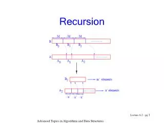
Recursion. Recursion. The recursion between all pairs of blocks can be solved in parallel. The recursion stops when the size of the subproblems is small and we can merge the very small blocks through a sequential algorithm in O (1) time.

Recursion
E N D
Presentation Transcript
Recursion Advanced Topics in Algorithms and Data Structures
Recursion • The recursion between all pairs of blocks can be solved in parallel. • The recursion stops when the size of the subproblems is small and we can merge the very small blocks through a sequential algorithm in O(1) time. • At the end of the algorithm, we know rank(B : A) and rank(A : B). Hence, we can move the elements to another array in sorted order. Advanced Topics in Algorithms and Data Structures
Complexity • The recursion satisfies the recurrences either : or, • The processor requirement is O(m + n). • The total work done is O(m + n) loglog m. Advanced Topics in Algorithms and Data Structures
An optimal merging algorithm • The make the algorithm optimal, we need to reduce the work to O(m + n). • We use a different sampling strategy and use the fast algorithm that we have designed. For simplicity, we assume that each array has n elements. • We divide the arrays A and B into blocks of size loglog n. • We choose the last element from each block as our sample and form two arrays A’ and B’. • Hence each of A’ and B’ has elements. Advanced Topics in Algorithms and Data Structures
Taking the samples • Now we compute rank(A’ : B’) and rank(B’ : A’) using the algorithm we have designed. • This takes O(loglog n) time and or O(n) work. Advanced Topics in Algorithms and Data Structures
Ranking the elements • We now compute rank(A’ : B) in the following ways. • Suppose the elements in A’ are: p1, p2,…, pn / loglog n. Advanced Topics in Algorithms and Data Structures
Ranking the elements • Consider pi A’. If rank(pi : B’) is the first element in block Bk, • Then rank(pi,B) must be some element in block Bk. • We do a binary search using one processor to locate rank(pi,B). Advanced Topics in Algorithms and Data Structures
Ranking the elements • We allocate one processor for pi. The processor does a binary search in Bk. • Since there are O(loglog n) elements in Bk, this search takes O(logloglog n) time. • The search for all the elements in A’ can be done in parallel and requires processors. • We can compute rank(B’ : A) in a similar way. Advanced Topics in Algorithms and Data Structures
Recursion again • Consider Ai, a loglog n block in A. • We know rank(p : B) and rank(q : B) for the two boundary elements p and q of Ai. • Now we can call our algorithm recursively with Ai and all the elements in B in between rank(p : B) and rank(q : B) . Advanced Topics in Algorithms and Data Structures
Recursion again • The problem is, there may be too many elements in between rank(p : B) and rank(q : B). • But then there are too many loglog n blocks in between rank(p : B) and rank(q : B) . Advanced Topics in Algorithms and Data Structures
Recursion again • The boundaries of all these blocks must be ranked in Ai. • Hence we get pairs of blocks, one loglog n block from B and a smaller block from Ai. Advanced Topics in Algorithms and Data Structures
Solving the subproblems • Now each of the two blocks participating in a subproblem has size at most loglog n. • And there are such pairs. • We assign one processor to each pair. This processor merges the elements in the pair sequentially in O(loglog n) time. • All the mergings can be done in parallel since we have processors. Advanced Topics in Algorithms and Data Structures
Complexity • Computing rank(A’ : B’) and rank(B’ : A’) take O(loglog n) time and O(n) work. • Computing rank(A’ : B) and rank(B’ : A) take O(loglog n) time and O(n) work. • The final merging also takes the same time and work. • Hence, we can merge two sorted arrays of length n each in O(n) work and O(loglog n) time on the CREW PRAM. Advanced Topics in Algorithms and Data Structures
An efficient sorting algorithm • We can use this merging algorithm to design an efficient sorting algorithm. • Recall the sequential merge sort algorithm. • Given an unsorted array, we go on dividing the array into two parts recursively until there is one element in each leaf. • We then merge the sorted arrays pairwise up the tree. • At the end we get the sorted array at the root. Advanced Topics in Algorithms and Data Structures
An efficient sorting algorithm • We can use the optimal merging algorithm to merge the sorted arrays at each level. • There are n elements in each level of this binary tree distributed among several arrays depending upon the level. • Hence we need O(loglog n) time and O(n) work for all the pairwise mergings at each level. • The binary tree has a depth of O(log n) . • Hence we can sort n elements in total work O(n log n) and time O(log n loglog n) Advanced Topics in Algorithms and Data Structures
Better sorting algorithms? • This sorting algorithm is work-optimal since the sequential lower bound for sorting is (n log n). • However, it is not time optimal. • Cole’s pipelined merge sort algorithm is an optimal O(log n) time and O(n log n) work sorting algorithm on the EREW PRAM. Advanced Topics in Algorithms and Data Structures