SOFT COMPUTING Evolutionary Computing
SOFT COMPUTING Evolutionary Computing. EC. What is a GA?. GAs are adaptive heuristic search algorithm based on the evolutionary ideas of natural selection and genetics. As such they represent an intelligent exploitation of a random search used to solve optimization problems.

SOFT COMPUTING Evolutionary Computing
E N D
Presentation Transcript
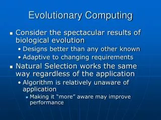
What is a GA? • GAs are adaptive heuristic search algorithm based on the evolutionary ideas of natural selection and genetics. • As such they represent an intelligent exploitation of a random search used to solve optimization problems. • Although randomized, GAs are by no means random, instead they exploit historical information to direct the search into the region of better performance within the search space.
What is a GA? • The basic techniques of the GAs are designed to simulate processes in natural systems necessary for evolution, specially those follow the principles first laid down by Charles Darwin of "survival of the fittest.". • Since in nature, competition among individuals for scanty resources results in the fittest individuals dominating over the weaker ones.
Evolutionary Algorithms Evolution Strategies Genetic Programming Genetic Algorithms Classifier Systems Evolutionary Programming • genetic representation of candidate solutions • genetic operators • selection scheme • problem domain
History of GAs • Genetic Algorithms were invented to mimic some of the processes observed in natural evolution. Many people, biologists included, are astonished that life at the level of complexity that we observe could have evolved in the relatively short time suggested by the fossil record. • The idea with GA is to use this power of evolution to solve optimization problems. The father of the original Genetic Algorithm was John Holland who invented it in the early 1970's.
Classes of Search Techniques DFS, BFS Tabu Search Hill Climbing Genetic Programming
Early History of EAs • 1954: Barricelli creates computer simulation of life – Artificial Life • 1957: Box develops Evolutionary Operation (EVOP), a non-computerised evolutionary process • 1957: Fraser develops first Genetic Algorithm • 1958: Friedberg creates a learning machine through evolving computer programs • 1960s, Rechenverg: evolution strategies • a method used to optimize real-valued parameters for devices • 1960s, Fogel, Owens, and Walsh: evolutionary programming • to find finite-state machines • 1960s, John Holland: Genetic Algorithms • to study the phenomenon of adaptation as it occurs in nature (not to solve specific problems) • 1965: Rechenberg & Schwefel independently develop Evolution Strategies • 1966: L. Fogel develops Evolutionary Programming as a means of creating artificial intelligence • 1967: Holland and his students extend GA ideas further
The Genetic Algorithm • Directed search algorithms based on the mechanics of biological evolution • Developed by John Holland, University of Michigan (1970’s) • To understand the adaptive processes of natural systems • To design artificial systems software that retains the robustness of natural systems • The genetic algorithms, first proposed by Holland (1975), seek to mimic some of the natural evolution and selection. • The first step of Holland’s genetic algorithm is to represent a legal solution of a problem by a string of genes known as a chromosome.
Evolutionary Programming • First developed by Lawrence Fogel in 1966 for use in pattern learning • Early experiments dealt with a number of Finite State Automata • FSA were developed that could recognise recurring patterns and even primeness of numbers • Later experiments dealt with gaming problems (coevolution) • More recently has been applied to training of neural networks, function optimisation & path planning problems
Biological Terminology • gene • functional entity that codes for a specific feature e.g. eye color • set of possible alleles • allele • value of a gene e.g. blue, green, brown • codes for a specific variation of the gene/feature • locus • position of a gene on the chromosome • genome • set of all genes that define a species • the genome of a specific individual is called genotype • the genome of a living organism is composed of several • chromosomes • population • set of competing genomes/individuals
Genotype versus Phenotype • genotype • blue print that contains the information to construct an • organism e.g. human DNA • genetic operators such as mutation and recombination • modify the genotype during reproduction • genotype of an individual is immutable • (no Lamarckian evolution) • phenotype • physical make-up of an organism • selection operates on phenotypes • (Darwin’s principle : “survival of the fittest”)
Courtesy of U.S. Department of Energy Human Genome Program , http://www.ornl.gov/hgmis
Genotype Operators • recombination (crossover) • combines two parent genotypes into a new offspring • generates new variants by mixing existing genetic material • stochastic selection among parent genes • mutation • random alteration of genes • maintain genetic diversity • in genetic algorithms crossover is the major operator • whereas mutation only plays a minor role
offspring A offspring B parent A parent B 1 1 0 1 0 1 1 0 1 1 1 0 0 0 1 0 1 0 0 0 0 offspring A offspring B 1 1 0 1 0 1 1 0 0 1 0 0 0 1 0 1 1 0 1 Crossover • crossover applied to parent strings with • probability pc : [0.6..1.0] • crossover site chosen randomly • one-point crossover • two-point crossover parent A parent B
offspring: 1 1 0 0 0 Mutate fourth allele (bit flip) mutated offspring: 1 1 1 0 0 0 Mutation • mutation applied to allele/gene with • probability Pm: [0.001..0.1] • role of mutation is to maintain genetic diversity
mutation population of genotypes 10011 10111 phenotype space f 01001 01001 10 10 10011 011 001 10001 01 01 01001 001 011 coding scheme 00111 11001 recombination selection 01011 10001 10001 x 01011 fitness 10001 11001 01011 Structure of an Evolutionary Algorithm
Pseudo Code of an Evolutionary Alg. Create initial random population Evaluate fitness of each individual yes Termination criteria satisfied ? stop no Select parents according to fitness Recombine parents to generate offspring Mutate offspring Replace population by new offspring
00101 00101 00101 00101 00101 01011 01011 01011 01011 01011 10001 10001 10001 10001 10001 11010 11010 11010 11010 11010 Roulette Wheel Selection • selection is a stochastic process • probability of reproduction pi = fi / Sk fk • selected parents :01011, 11010, 10001, 10001
Genetic Programming • automatic generation of computer programs • by means of natural evolution see Koza 1999 • programs are represented by a parse tree (LISP expression) • tree nodes correspond to functions : • - arithmetic functions {+,-,*,/} • - logarithmic functions {sin,exp} • leaf nodes correspond to terminals : • - input variables {X1, X2, X3} • - constants {0.1, 0.2, 0.5 } + X1 * tree is parsed from left to right: (+ X1 (* X2 X3)) X1+(X2*X3) X2 X3
- + X2 / X1 * - X1 X2 X3 X2 X3 Genetic Programming : Crossover parent A parent B - * / + offspring B offspring A X2 X3 X2 X1 - X1 X2 X3
Design of electronic circuits Telecommunication network design Artificial intelligence Study of atomic clusters Study of neuronal behaviour Neural network training & design Automatic control Artificial life Scheduling Travelling Salesman Problem General function optimisation Bin Packing Problem Pattern learning Gaming Self-adapting computer programs Classification Test-data generation Medical image analysis Study of earthquakes Areas EAs Have Been Used In
Goldberg (1989) • Goldberg D. E. (1989), Genetic Algorithms in Search, Optimization, and Machine Learning. Addison-Wesley, Reading.
Michalewicz (1996) • Michalewicz, Z. (1996), Genetic Algorithms + Data Structures = Evolution Programs, Springer.
Vose (1999) • Vose M. D. (1999), The Simple Genetic Algorithm : Foundations and Theory (Complex Adaptive Systems). Bradford Books;
Genetic Fuzzy Systems (GFS’s) • genetic design of fuzzy systems • automated tuning of the fuzzy knowledge base • automated learning of the fuzzy knowledge base • objective of tuning/learning process • optimizing the performance of the fuzzy system: • e.g.: fuzzy modeling : minimizing quadratic error • between data set and the fuzzy system outputs • e.g : fuzzy control system: optimize the • behavior of the plant + fuzzy controller
Genetic Fuzzy System for Data Modeling fitness Evolutionary algorithm Evaluation scheme genotype Fuzzy system parameters phenotype Fuzzy System Dataset : xi,yi
Database : Definition of fuzzy membership- function Rule base: definition of fuzzy rules If X1 is A1 and … and Xn is An then Y is B a b c Fuzzy Systems Knowledge Base
Genetic Tuning Process • tuning problems utilize an already existing rule base • tuning aims to find a set of optimal parameters for • the database : • points of membership-functions [a,b,c,d] • or • scaling factors for input and output variables
a0 b0 a1 b2*(n+1) . . . 100101 011111 110101 100101 a0 b0 a1 b2*(n+1) . . . x0,so x1,s1 x2,s2 xm,sm Linear Scaling Functions • Chromosome for linear scaling: • for each input xi : two parameters ai,bi i=1..n • for the output y : two parameter a0,b0 • Genetic Algorithms: • encode each parameter by k bit using Gray code • total length = 2*(n+1)*k bit • Evolutionary Strategies: • each parameter ai or bi corresponds to one • object variable xm m : 1… 2*(n+1)
Descriptive Knowledge Base • descriptive knowledge base m m neg ze pos sm me lg y x • all rules share the same global membership functions : • R1 : if X is sm then Y is neg • R2 : if X is me then Y is ze • R3 : if X is lg then Y is pos
R1 : if X is then Y is Approximate Knowledge Base • each rule employs its own local membership function R1 : if X is then Y is R1 : if X is then Y is R1 : if X is then Y is • tradeoff: more degrees of freedom and therefore • better approximation but intuitive meaning of • fuzzy sets gets lost
Tuning Membership Functions • encode each fuzzy set by characteristic parameters Trapezoid: <a,b,c,d> Gaussian: N(m,s) (x) (x) 1 1 s 0 0 a b c d x m x Triangular: <a,b,c> (x) 1 0 a b c x x
Approximate Genetic Tuning Process • a chromosome encodes the entire knowledge base, • database and rulebase Ri : if x1 is Ai1 and … xn is Ain then y is Bi encoded by the i-th segment Ci of the chromosome using triangular membership-functions (a,b,c) = Ci (ai1, bi1, ci1, . . . , ain, bin, cin, ai, bi, ci, ) each parameter may be binary or real-coded The chromosome is the concatenation of the individual segments corresponding to rules : C1 C2 C3 C4 Ck . . .
Descriptive Genetic Tuning Process • the rule base already exists • assume the i-th variable is composed of Ni terms = Ci (ai1, bi1, ci1, . . . , aiNi, biNi, ciNi ) m A1 A2 A3 xi ai1, bi1, ci1, ai2, bi2, ci2 ai3, bi3, ci3 The chromosome is the concatenation of the individual segments corresponding to variables : C1 C2 C3 C4 Ck . . .
Descriptive Genetic Tuning • in the previous coding scheme fuzzy sets might • change their order and optimization is subject • to the constraints : aij < bij < cij A1 A2 A3 x1 x2 x3 • encode the distance among the center points • of triangular fuzzy sets and choose the border • points such that Smi = 1
Fitness Function for Tuning • minimize quadratic error among training data (xi,yi) • and fuzzy system output f(xi) • E = Sumi (yi-f(xi))2 • Fitness = 1 / E (maximize fitness) • minimize maximal error among training data (xi,yi) • and fuzzy system output f(xi) • E = maxi (yi-f(xi))2 • Fitness = 1 / E (maximize fitness)
Genetic Learning Systems • genetic learning aim to : • learn the fuzzy rule base • or • learn the entire knowledge base • three different approaches • Michigan approach : each chromosome represents • a single rule • Pittsburgh approach : each chromosome represents • an entire rule base / knowledge base • Iterative rule learning : each chromosome represents • a single rule, but rules are injected one after the • other into the knowledge base
Michigan Approach Population: Individual: 11001 : R1: if x is A1 ….then Y is B1 00101 : R2: if x is A2 ….then Y is B2 10111 : R3: if x is A3 ….then Y is B3 11100 : R4: if x is A4 ….then Y is B4 01000 : R5: if x is A5 ….then Y is B5 11101 : R6: if x is A6 ….then Y is B6 B4 X Y B5 A4 A1 B1 A5 A3 B6 A2 A6 B2 B3
R1 : if x is large then Y is neg. R2 : if x is med. then Y is zero F = 2.5 F=2.7 R3 : if x is small then Y is zero R4 : if x is small then Y is pos. F=-0.4 F=-1.6 Cooperation vs. Competition Problem • we need a fitness function that measures the • accuracy of an individual rule as well as the • quality of its cooperation with other rules Fitness = number of correct classifications minus number of incorrect classifications Y pos ze neg small medium large X
competitors: 11001 : R1: if x is A1 ….then Y is B1 10111 : R3: if x is A3 ….then Y is B3 11100 : R4: if x is A4 ….then Y is B4 removed from the population Michigan Approach • steady state selection: • pick one individual at random • compare it with all individuals that cover • the same input region • remove the “relatively” worst one from the • population • pick two parents at random independent of • their fitness and generate a new offspring 11001 : R1: if x is A1 ….then Y is B1 00101 : R2: if x is A2 ….then Y is B2 10111 : R3: if x is A3 ….then Y is B3 11100 : R4: if x is A4 ….then Y is B4 01000 : R5: if x is A5 ….then Y is B5 11101 : R6: if x is A6 ….then Y is B6
Thanks for your attention! That’s all.