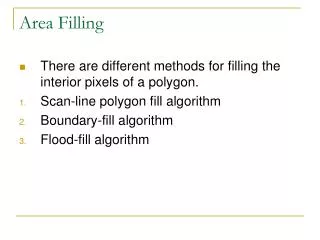
Area Filling
Area Filling. There are different methods for filling the interior pixels of a polygon. Scan-line polygon fill algorithm Boundary-fill algorithm Flood-fill algorithm. 9. 8. e 2. e 3. 7. e 4. 6. e 1. 5. 4. 3. 2. e 5. 1. e 6. 0. 0. 1. 2. 3. 4. 5. 6. 7. 8. 9. 10.

Area Filling
E N D
Presentation Transcript
Area Filling • There are different methods for filling the interior pixels of a polygon. • Scan-line polygon fill algorithm • Boundary-fill algorithm • Flood-fill algorithm
9 8 e2 e3 7 e4 6 e1 5 4 3 2 e5 1 e6 0 0 1 2 3 4 5 6 7 8 9 10 Scan line approach To fill the area, we can work in scan lines. Take a y-value; find intersections with edges. Join successive pairs filling in a span of pixels
9 8 e2 e3 7 e4 6 e1 5 4 3 2 e5 1 e6 0 0 1 2 3 4 5 6 7 8 9 10 Different Cases - the normal case Scan line 5: intersection e1 = 1.14 intersection e4 = 8.5 Pixels 2-8 on scan line are filled in
9 8 e2 e3 7 e4 6 e1 5 4 3 2 e5 1 e6 0 0 1 2 3 4 5 6 7 8 9 10 Different Cases - Passing through a vertex Scan line 6 intersects e1,e2,e3,e4 at 1.4, 4, 4, 8 respectively - two spans drawn Scan line 4 intersects e1,e4,e5 at 0.9, 9, 9 respectively - when edges are either side of scan line, just count upper ie e4
9 8 e2 e3 7 e4 6 e1 5 4 3 2 e5 1 e6 0 0 1 2 3 4 5 6 7 8 9 10 Different cases - horizontal edges A horizontal edge such as e6 can be ignored; it will get drawn automatically
9 8 e2 e3 7 e4 6 e1 5 4 3 2 e5 1 0 0 1 2 3 4 5 6 7 8 9 10 Pre-Processing the Polygon We have removed e6, and shortened e5 by one scan line
9 8 e2 e3 7 e4 6 e1 5 4 3 2 e5 1 0 0 1 2 3 4 5 6 7 8 9 10 Optimization To speed up the intersection calculations it helps to know where the edges lie: eg e1 goes from scan line 1 to scan line 8; e2 from line 8 to line 6 Thus we know which edges to test for each scan line
9 8 e2 e3 7 e4 6 e1 5 4 3 2 e5 1 0 0 1 2 3 4 5 6 7 8 9 10 Bucket Sort the Edges In fact it is useful to sort the edges by their lowest point; we do this by bucket sort - one bucket per scan line 0: 1: e1,e5 2: 3: 4: e4 5: 6: e2,e3 7: 8: 9:
9 8 e2 e3 7 e4 6 e1 5 4 3 2 e5 1 0 0 1 2 3 4 5 6 7 8 9 10 Next Optimization - Using Coherence The next optimization is to use scan line coherence Eg. look at e1 - assume intersection with line 1 known (x=0) - then intersection with scan line 2 is: x = x + 1/m (m=slope) ie: x = x + Dx / Dy ie: x = 0 + 2 / 7 = 2/7 Dy Dx
9 8 e2 e3 7 e4 6 e1 5 4 3 2 e5 1 0 0 1 2 3 4 5 6 7 8 9 10 Creating An Edge Table It is useful to store information about edges in a table: Dy Max y e 1st x Dx 1 0 8 2 7 4 8 -2 2 2 3 4 5
9 8 e2 e3 7 e4 6 e1 5 4 3 2 e5 1 0 0 1 2 3 4 5 6 7 8 9 10 An Efficient Polygon Fill Algorithm (1) Set y = 0 (2) Check y-bucket (3) Add any edges in bucket to active edge table (AET) (4) If AET empty, then set y = y + 1, and go to (2)
9 8 max y e2 e3 e x Dx Dy 7 e4 2 7 6 1 0 8 e1 5 5 6 3 2 2 4 3 2 e5 1 0 0 1 2 3 4 5 6 7 8 9 10 Active Edge Table y = 1 (5) Put x-values in order and fill in between successive pairs
9 8 e2 e3 7 e4 6 e1 5 4 max y 3 e x Dx Dy 2 e5 2 7 1 2/7 8 1 5 7 3 2 2 0 0 1 2 3 4 5 6 7 8 9 10 Active Edge Table (5) Set y = y+1; remove any edge from active table with ymax < y (6) Increment x by Dx / Dy y = 2 (7) Return to (2)
9 8 e2 e3 7 e4 6 e1 5 4 3 2 e5 1 0 0 1 2 3 4 5 6 7 8 9 10 Next Scan Line At each stage of the algorithm, a span (or spans) of pixels are drawn
Working in Integers • The final efficiency step is to work in integer arithmetic only - this needs an extra column in the AET as we accumulate separately the whole part of x and its fractional part
Working in Integers First intersection is at x=0, and the slope of the edge is 7/2 - ie DY=7, DX=2 The successive intersection points are: 0 2/7 4/7 6/7 8/7 etc The corresponding starting pixels for scan line filling are: 0 0 0 0 1 We can deduce this just by adding DX at each stage, until DY reached at which point DX is reduced by DY: 0 2 4 6 1 (8-7) etc
9 max y e x Dx Dy 8 e2 e3 7 2 7 1 0 8 e4 6 5 6 3 2 2 e1 5 4 3 2 e5 1 0 0 1 2 3 4 5 6 7 8 9 10 Integer Active Edge Table y = 1 becomes x int x frac max y Dx Dy e 1 0 0 8 2 7 5 6 0 3 2 2
9 8 e2 e3 7 e4 6 e1 5 4 3 2 e5 1 0 0 1 2 3 4 5 6 7 8 9 10 Integer Active Edge Table At step (7), rather than increment x by Dx/Dy, we increment x-frac by Dx; whenever x-frac exceeds Dy, we add 1 to x-int & reduce x-frac by Dy y = 2 x int x frac max y Dx Dy e 1 0 2 8 2 7 5 7 0 3 2 2
9 8 e2 e3 7 e4 6 e1 5 4 3 x int x frac max y Dx Dy e 2 e5 1 1 0 4 8 2 7 0 5 8 0 3 2 2 0 1 2 3 4 5 6 7 8 9 10 The next step is We increment x-frac by Dx; whenever x-frac exceeds Dy, we add 1 to x-int & reduce x-frac by Dy y = 3 Notice: X is the same as the previous scan.
Data Structures • Edge: A record structure that represents an edge of the polygon. • Edge Table ET: An array of lists of edges. It represents the whole polygon. • Active Edge Table AET: A linked list of edges. It represents the edges that intersect the current scan line.
Edge Structure • YMAX (int) Field: The y coordinate of the higher of the two endpoints of the edge. • X (float) Field: Initially the x coordinate of the lower endpoint of the edge. Later, the x coordinate of the intersection of the edge with the current scan line. • INVSLOPE (float) Field: The reciprocal of the slope of the edge. • NEXT (edge*) Field: A pointer to the next edge on a linked list of edges.
Edge Table (ET) • ET holds all the non-horizontal edges. • ET is an array indexed by scan lines. • Each array element ET[y] is a linked list of edges. • Each edge on the list ET[y] has y as the vertical coordinate of the lower of its two endpoints.
Active Edge Table (AET) • AET is initially empty. • AET always holds a list of the non-horizontal edges that intersect the current scan line. • The edges in AET are sorted according to the x coordinate of their intersections with the current scan line.
Polygon Filling Algorithm 1. Initialize ET and AET; 2. Let the current scan line y be the index of the first entry in ET pointing to a non-empty edge list. 3. While (y ≤ Max Scan Line) and (ET or AET not empty) do: a. Remove from AET each edge E with Y=E.YMAX. b. For each edge E in AET do E.X = E.X + E.INVSLOPE. c. Move each edge in ET[y] to AET. d. Sort the edges in AET by the value of the X field. e. Fill spans whose endpoints are given by the X fields of successive pairs of edges in AET. f. Increment y, the current scan line.
Area filling algorithms • Both boundary-fill algorithm & flood-fill algorithm need to identify one interior point. • Odd-even rule is used to test if a point P is inside a given polygon or outside it. • The rule: • Pick a point q outside the polygon. (How?) • Join p and q with a line L • Find and count points of intersections between L and polygon edges. • If one of the points of intersection is a vertex v is shared between two edges e1 and e2, then if the other two ends of e1 and e2 are in opposite directions of L, then count this point once otherwise count it two. • If number of points is odd then P is inside otherwise it is outside.
Boundary fill algorithm • Starting from a point inside the polygon, paint the points outward towards the boundary. • There are two methods to proceed to neighboring pixels from the current one. • 4 neighboring points are tested: left, right, above, and below. • May not work in some cases. • 8 neighboring points: the above 4 in addition to the two diagonal point.
Boundary fill algorithm // Input: – Boundary Color (BC), Fill Color (FC) – (x,y) coordinates of seed point known to be inside BndFill(x,y,BC,FC) { color = GetPixel(x,y) if ( (color != BC) && (color != FC) ) { SetPixel(x,y,FC); BndFill(x+1,y,BC,FC); BndFill(x,y+1,BC,FC); BndFill(x-1,y,BC,FC); BndFill(x,y-1,BC,FC); } }
Flood Fill Algorithm • Fill area identified by the interior color instead of boundary color • Good for single colored area with multicolor border • Can be used for arbitrary areas! • BUT • Deep Recursion so: Uses enormous amounts of stack space • Also very slow since: Extensive pushing/popping of stack • Pixels may be visited more than once • GetPixel() & SetPixel() called for each pixel
The algorithm // Input: – Old Color (OC), Fill Color (FC) – (x,y) coordinates of seed point known to be inside BndFill(x,y,OC,FC) { color = GetPixel(x,y) if ( color == OC ) { SetPixel(x,y,FC); BndFill(x+1,y,BC,FC); BndFill(x,y+1,BC,FC); BndFill(x-1,y,BC,FC); BndFill(x,y-1,BC,FC); } }