Download
1 / 51
570 likes | 1.03k Vues
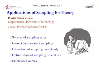
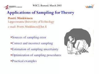
Applications of Sampling for Theory. Pentti Minkkinen. Lappeenranta University of Technology. e-mail: Pentti.Minkkinen@lut.fi. WSC2, Barnaul, March 2003. Sources of sampling error Correct and incorrect sampling Estimation of sampling uncertainty Optimization of sampling procedures

E N D
Applications of Sampling for Theory Pentti Minkkinen Lappeenranta University of Technology e-mail: Pentti.Minkkinen@lut.fi WSC2, Barnaul, March 2003 • Sources of sampling error • Correct and incorrect sampling • Estimation of sampling uncertainty • Optimization of sampling procedures • Practical examples
LOT m (s) Primary Secondary Analysis Result sample sample s1s2s3sx x Propagation of errors: Example: GOAL: x = m Analytical process usually contains several sampling and sample preparation steps
SAMPLING • Art of cutting a small portion of material from a large lot and transferring it to the analyzer • Theory of sampling (theoretical) distributions with known properties • SLOGANS • The result is not better than the sample that it is based on • Sample must be representative • Theory that combines both technical and statistical parts • of sampling has been developed by Pierre Gy: • Sampling for Analytical Purposes, Wiley, 1998
PLANNING OF SAMPLING • GATHERING OF INFORMATION • What are the analytes to be determined? • What kind of estimates are needed? • Average (hour, day, shift, batch, shipment, etc.) • Distribution (heterogeneity) of the determinand in the lot • Highest or lowest values • Is there available useful a priory information (variance estimates, unit costs)? • Is all the necessary personnel and equipment available? • What is the maximum cost or uncertainty level of the investigation?
PLANNING OF SAMPLING • 2. DECISIONS TO BE MADE • Manual vs. automatic sampling • Sampling frequency • Sample sizes • Sampling locations • Individual vs. composite samples • Sampling strategy • Random selection • Stratified random selection • Systematic stratified selection • Training
Global Estimation Error GEE Total Sampling Error TSE Total Analytical Error TAE Point Materialization Error PME Weighting Error SWE Increment Extraction Error IXE Increment Delimi- tationError IDE Increment and Sample Preparation Error IPE Point Selection Error PSE Long Range Point Selection Error PSE1 Periodic Point Selection Error PSE2 Grouping and Segregation Error GSE Fundamental Sampling Error FSE GEE=TSE +TAE TSE= (PSE+FSE+GSE)+(IDE+IXE+IPE)+SWE Error components of analytical determination according to P.Gy
Sample Ideal mixing If the lot to be sampled can be mixed before sampling it can be treated as a 0-dimensional lot. Fundamental sampling error determines the correct sampling errorand can be estimated by using binomial or Poisson distributions as models, or by using Gy’s fundamental sampling error equations. 0-D
1-D Samples 2-D If the lot cannot be mixed before sampling the dimensionality of the lot depends on how the samples are delimited and cut from the lot. Auto- correlation has to be taken into account in sampling error estimation
Samples 3-D Lot is 3-dimensional, if none of the dimensions is completely included in the sample
Weighting error Concentration Volume c·V Sample 3 No. mg/l m g 6.25 4.58 28.6 1 4.36 3.71 16.2 2 5.58 5.20 28.99 3 4.64 5.71 26.48 4 4.86 4 .54 22.08 5 3.65 6.78 24.75 6 3.73 7.12 26.55 7 5.98 5.81 34.76 8 4.96 5.86 29.05 9 4.89 5.479 26.39 Mean Sum 44.01 49.3 237.47 å Weighted mean concentration: = 4.86 mg/l å Vi Totalemission estimate (unweighted): 241.13 = × × = × × × × = 3 3 M 9 c V 9 4 . 89 g / m 5 . 479 m = × × = × × × × = 3 3 237.47 g M 9 c V 9 4 . 86 g / m 5 . 479 m Total emission estimate (weighted): w w Weighting error (in concentration):0.03 mg/l Weighting error (in total emission):3.66 g ciVi
v a b c Correct design for proportional sampler:correct increment extraction v= constant 0.6 m/s if d > 3 mm, b 3d = b0 ifd < 3 mm,b 10 mm = b0 d = diameter of largest particles b0 = minimum opening of the sample cutter
Incorrect Increment and Sample Preparation Errors • Contamination (extraneous material in sample) • Losses (adsorption, condensation, precipitation, etc.) • Alteration of chemical composition (preservation) • Alteration of physical composition (agglomeration, breaking of particles, moisture, etc.) • Involuntary mistakes (mixed sample numbers, lack of knowledge, negligence) • Deliberate faults (salting of gold ores, deliberate errors in increment delimitation, forgery, etc.)
Estimation of Fundamental Sampling Error by Using Poisson Distribution • Poisson distribution is describes the random distribution of rare • events in a given interval. • If msis the number of critical particles in sample, the standard • Deviation expressed as the number of particles is (1) • The relative standard deviation is (2)
Example Plant Manager:I am producing fine-ground limestone that is used in paper mills for coating printing paper. According to their speci- fication my product must not contain more than 5 particles/tonne particles larger than 5 mm. How should I sample my product? Sampling Expert:That is a bit too general a question. Let’s first define our goal. Would 20 % relative standard deviation for the coarse particles be sufficient? Plant Manager: Yes. Sampling Expert:Well, let’s consider the problem. We could use the Poisson distribution to estimate the required sample size. Let’s see:
The maximum relative standard deviation sr = 20 % = 0.2. From equation2 we can estimate how many coarse particles there should be in the sample to have this standard deviation If 1 tonne contains 5 coarse particles this result means that the primary sample should be 25 tonnes. This is a good example of an impossible sampling problem. Even though you could take a 25 tonne sample there is no feasible technology to separate and count the coarse particles from it. You shouldn’t try the traditional analytical approach in con-trolling the quality of your product. Instead, if the specification is really sensible, you forget the particle size analyzers and maintain the quality of your product by process technological means, that is, you take care that all equipment are regularly serviced and their high performance maintained to guarantee the product quality. Plant Manager: Thank you
if Ms << ML where = relative standard deviation Ms= sample size ML = lot size d = particle size (95 % top size) aL = average concentration of the analyte in the lot C = Sampling constant P.Gy’s Fundamental sampling error model
composition factor liberation factor size distribution factor shape factor SAMPLING CONSTANT C
default in most cases d d d d f= 0,5 f= 0,1 f= 1 f= 0,524 L = d Estimation of shape factor d L Estimation of liberation factor for unliberated and liberated particles
Estimation of size distribution factor, g Wide size distribution (d/d0.05 > 4) defaultg = 0.25 Medium distribution (d/d0.05 = 4...2) g = 0.50 Narrow distribution (1 < d/d0.05 < 2) g = 0.75 Identical particles (d/d0.05 = 1) g = 1.00
Estimation of constitution factor, c density of critical particles average concentration of the lot density of matrix concentration of determinand in critical particles
Example: A chicken feed (density = 0.67 g/cm3) contains as an average 0.05 % of an enzyme powder that has a density of 1.08 g/cm3. The size distribution of the enzyme particle size d=1.00 mm and the size range factor g = 0.5 could be estimated. Estimate the fundamental sampling error for the following analytical procedure. First a 500 g sample is taken from a 25 kg bag. This sample is ground to a particle size -0.5 mm. Then the enzymeis extracted from a 2 g sample by using a proper solvent and the concentration is determined by using liquid chromatography. The relative standard deviation of the chromatographic measurement is 5 %.
Total relative standard deviation: ML =25000 g; d = 1 mm rc = 1.08 g/cm3 ; a = 100 % ; b = 1 rm = 0.67 g/cm3 ; aL = 0.05 % ; f = 0.5 c =2160 g/cm3 d 1= 1 mm; MS1 = 500 g ; ML1 =25000 g; g 1 = 0.5; C 1= 540 g/cm3 sr1 = 0.033 =3.3 % (primary sample) • d 2= 0.5 mm; MS2 =2 g ; ML2 =500 g; g 2 = 0.25; • C 1= 270 g/cm3 • sr2 = 0.13 =13 % (secondary sample) sr3 = 0.05 = 5 % (analysis)
Analysis of Mineral Mixtures by Using IR Spectrometry Pentti Minkkinena), Marko Lalloa), Pekka Stenb), and Markku J. Lehtinenc) a) Lappeenranta University of Technology, Department of Chemical Technology, P.O. Box 20, FIN-53851 Lappeenranta, Finland b) Technical Research Centre of Finland (VTT), Chemical Technology, Mineral Processing, P.O. Box 1405, FIN-83501 Outokumpu, Finland c) Partek Nordkalk Oy Ab, Poikkitie 1, FIN-53500 Lappeenranta, Finland (Present address: Geological Survey of Finland, R & D Department/Mineralogy and Applied Mineralogy, P.O.Box 96, FIN-2151 Espoo, Finland)
Content • Introduction • Sampling error estimation and sample preparation • Design of calibration and test sets • Calibration (PLS) • Results
Introduction • In mineral processing it is important to know quanti-tatively the mineral composition of the material to be processed • The methods presently in use time consuming • Only a few reports in literature on use of IR for mineral analysis • Feasibility of FTIR (Nicolet Magna 560) to analyze quantitatively mineral species associated with wollastonite was studied
Design of calibration set • Mixture design for five components by using XVERT- algorithm (CORNELL, J.A., Experi-ments with Mixtures, 2nd Edition, Wiley, 1990, pp 139-227) • 37 calibration and 5 validation standards
Calibration • Spectra recorded with Nicolet Magna 560 FTIR spectrometer • Calibration with PLS1 (model calculated by using TURBOQUANT program)
PREPARATION OF CALIBRATION STANDARDS • Pure minerals (d=1mm) were ground individually 2 min in a swing mill • 30 mg-2.95 g of each mineral were carefully weighted to obtain the designed composition which was carefully mixed 3 min in a Retsch Spectro Mill • 20 mg of the mineral mixture was carefully weighted into 4.98 g of KBr and mixed 3 min in a Retsch Spectro Mill • 200 mg of the mineral-KBr mixture was pressed into a tablet for the IR measurement
Sampling errors of sample preparation and IR measurement Dilution factor = = 0.004 Tablet Preparation: Lot size = ML1 = 5 g Sample size = Ms1 = 0.2 g IR Measurement: Lot size = ML2 = 200 mg Sample size = Ms2 = 38% of 0.2 g = 76 mg
10 8 s r1 % 6 s r2 % 4 s rt % 2 0 1 2 3 4 5 6 7 8 9 10 Quartz concentration (%) RESULTS FSE of quartz determination
0.8 s r1 % 0.7 s r2 % 0.6 s rt % 0.5 0.4 80 82 84 86 88 90 92 94 96 Wollastonite concentration (%) FSE of wollastonite determination
QUARTZ 12 10 8 PREDICTED (%) 6 4 2 0 0 2 4 8 10 12 6 DESIGN (%) Experimental result (PLS-calibration) Designed vs. predicted concentration * = calibration, o = test set
WOLLASTONITE 96 94 92 90 88 PREDICTED (%) 86 84 82 80 78 76 78 80 82 84 86 88 90 92 94 96 DESIGN (%) Designed vs. predicted concentration * = calibration, o = test set
Conclusions • FTIR and PLS can be used for mineral analysis • Design and preparation of the calibration set important; pure minerals hard to get and vary in composition from deposit to deposit and also within a deposit • Reproducible sample preparation important both from the spectroscopic point of view and to control the sampling error • Still difficult for a routine laboratory
Uses of Gy’s fundamental sampling error model • srof a given sample size • Minimum Ms for a required sr • Maximum d for given Ms and sr • Audit and design of multistep sampling procedures
Estimation of point selection error, PSE PSE is the error of the mean of a continuous lot estimated by using discrete samples. • PSEdepends on sample selection strategy, if consecutive values are autocorrelated. Selection options: • random • stratified random • stratifiedsystematic. • Point selection error has two components: PSE = PSE1 + PSE2 • PSE1... error component caused by random drift • PSE2... error component caused by cyclic drift Statistics of correlated series is needed to evaluate the sampling variance.
100 Random selection 50 CONCENTRATION 0 0 5 10 15 20 25 30 TIME 100 Stratified selection 50 CONCENTRATION 0 0 5 10 15 20 25 30 TIME 100 CONCENTRATION Systematic selection 50 0 0 5 10 15 20 25 30 TIME
Random sampling: Stratified sampling: Systematic sampling: When sampling autocorrelated series the same number of samples gives different uncertainties for the mean depending on selection strategy sp is the process standard deviation, sstr and ssys standard deviation estimates where the autocor-relation has been taken into account. Normallysp > sstr > ssys , except in periodic processes, where ssys may be the largest
, Heterogeneity of the process: , Estimation of PSE by variography Variogaphic experiment: Nsamples collected at equal distances Variogram of heterogeneity calculated: To estimate variances the variogram has to be integrated (numerically in Gy’s method)
0.015 A 0.01 V 0.005 0.04 B 0.02 V 0 0.02 C V 0.01 0 0.02 D 0.01 V 0 0 5 10 15 20 25 30 35 40 45 50 SAMPLE INTERVAL Shapes of variograms: A. Random process; B. Process with non-periodic drift; C. Periodic process; D. Complex process
1 0.5 hi 0 0.5 0 5 10 15 20 25 30 DAYS Estimation of sulfur in wastewater stream Heterogeneity of the process, sp = 0.282 =28.2 %
0.15 0.1 Vi 0.05 0 0 2 4 6 8 10 12 14 16 Sample interval (d) Variogram of sulfur in wastewater stream
25 20 s str sr (%) 15 s sys 10 5 0 0 5 10 15 Sample interval (d) Relative standard deviation estimates, which take auto- correlation into account
Standard deviation of the annual mean= Expanded uncertainty = Process standard deviation was 28.2 %.If the number of samples is estimated by using normal approximation (or samples are selected completely randomly) the required number of samples is for the same uncertainty: Estimate the uncertainty of the annual mean, if one sample/ week is analyzed by using systematic sample selection Sampling interval = 7 d ssys = 7.8 % Number of samples/y = n =52
CONCLUSIONS • Sampling uncertainty can be, and shouldbe estimated • If the sampling uncertainty is not known it is questionable • whether the sample should be analyzed at all • Sampling nearly always takes a significant part of the • total uncertainty budget • Optimization of sampling and analytical procedures may • result significant savings, or better results, including • scalesfrom laboratory procedures and process sampling • to large nationalsurveys