Download
1 / 16
160 likes | 308 Vues
The project : “ Numerical experiments on the natural convection Inside coaxial cylinders and concentric spheres” ( NUM-EXP-NAT-CONV). Bejo Duka Ergys Rexhepi Department of Physics, Faculty of Natural Sciences , UNIVERSITY OF TIRANA. Problem importance

E N D
The project:“Numerical experiments on the natural convection Inside coaxial cylinders and concentric spheres” (NUM-EXP-NAT-CONV) BejoDuka ErgysRexhepi Department of Physics, Faculty of Natural Sciences, UNIVERSITY OF TIRANA
Problem importance Natural convection of a fluid between rigid boundaries kept at constant surface temperature received much attention because of the theoretical interest and the wide engineering applications. The fluid flow in a cylindrical annulus shows a multiplicity of solutions (bifurcation phenomenon) [1], [2]. The problem of the stability of the solutions in different geometries (cylindrical or spherical) is at the uttermost interest of several theoretical studies [3][6]. In the case of two coaxial cylinders, using the Oberbeck-Boussinesq approximation[4], the partial differential equations governing conservation of mass, momentum and energy are written into non dimensional form of cylindrical coordinates introducing Prandtl and Rayleigh number [7]. References [1] C. Kim, and T.Ro, "Numerical Investigation on Bifurcative Natural Convection in an Air-Filled Horizontal Annulus", J. Heat Transfer, Vol.116, pp. 135-141, 1994. [2] J. D. Chung, C.-J. Kim, H. Yoo, J. S. Lee, “Numerical investigation on the bifurcative natural convection in a horizontal concentric annulus”, Numerical Heat Transfer, A, 36(1999), 291 - 307, [3]B. Duka, C. Ferrario, A. Passerini, S. Piva,“Non-linear approximations for natural convection in a horizontal annulus” , International Journal of Nonlinear Mechanics, 42 (2007), p. 1055-1061 [4] A. Passerini, G. Thäter, “Boussinesq-type approximation for second-grade fluids”, Int. J. Non-Linear Mech. 40 (2005) 821. [5] C. Ferrario, A. Passerini, S. Piva. Galdi, A Stokes-like system for natural convection in a horizontal annulus, Nonlinear Analysis: Real World Applications, Volume 9, Issue 2, April 2008, 403-411[6] C. Ferrario et al. "Theoretical results on steady convective flows between horizontal coaxial cylinders. siam j. appl. math, vol. 71, no. 2 ,2011, pp. 465–486. [7] Yoo, J.S., “Natural Convection in a Narrow Horizontal Cylinder Annulus: Pr <0.3”, Int. . Heat Mass Transfer, Vol. 41 (1998), pp. 3055-3073.
Previous Calculations In the Oberbeck- Boussinesq approximation (0 [1+(T-T0)] , the PDE system of equation are written: ∇ · v =0 (1/Pr) v · ∇v − v + ∇Π= (Ra /B)sin ϕer+ Ra τ e3 v · ∇τ − τ = vr / rB, where the Prandtl number and Rayleigh number are: Pr = ν/ k , Ra = (αg/νk)(Ti− To)(Ro− Ri )3 while B= ln(Ro/Ri) endowed with the boundary conditions v = 0, τ = 0 on ∂A (is the temperature deviation from the conduction profile) . Running ANSYS-Fluent software package (noncommercial version) in a PC, we studied the stability of solutions for different values of Prandtl and Rayleigh parameters and for different temperature difference between concentric cylinders. The calculations were limited by the PC capacities. For example to get solution presented here by the animation of streamlines, the calculation in a PC ended after one day. Therefore we applied the project: to run the numerical calculation in HP-SEE grids.
Preliminary calculations • The open source software that could substitute the ANSYS Fluent software for the numerical calculations in the field of CFD, is OpenFoam (Open Source Field Operation and Manipulation): • - Uses C++ libraries to solve numerically PDE • - Has several pre-build numerical solvers and pre/post processors too • - Is free under pubic license GNU • - Can be executed in parallel. • Is always in development by OpenFoam community. • We installed OpenFoam package (version 2.1.1 for CentOS) and its add-ins (post - processing utility, named “Paraview”) in our server (RedHat). We explored its capabilities aiming to carry out numerical experiments previewed by our project and executed some cases of its tutorial in serial mode. • Replying to our request, the administrator of the PARADOX cluster (Serbia), where our project is hosted, installed of the OpenFoam package and Paraview and offered the assistance for using it. • Thanks to the instructions and assistance of the Serbian specialist Vladimir Slavic, we have started to use OpenFoam known applications in the parallel mode. • As the internet connection to that cluster is very slow, we can’t visualize the results by the graphical mode log-in in Paradox claster. Therefore, after executing an OpenFoam case, we download the results and visualize them locally in our server.
Basics of OpenFoam OpenFOAM package uses FV (Finite Volume) method to solve numerically partial differential equations. Spatial discretisation means approximation of a problem into discrete quantities . Likes as the finite element and finite difference methods, the FV method defines the solution domain by a set of points that fill and bound a region of space (domain). Temporal discretisation (For transient problems) dividing the time domain into into a finite number of time intervals, or steps; Equation discretisation: Generating a system of algebraic equations in terms of discrete quantities defined at specific locations in the domain, from the PDEs that characterise the problem. Discretisation of the solution domain Discretisation of the solution domain is shown in Figure. The space domain is discre-tised into computational mesh on which the PDEs are subsequently discretised. Discretisation of time, if required, is simple: it is broken into a set of time steps tthat may change during a numerical simulation.Discretisation of space requires the subdivision of the domain into a number of cells, or control volumes. The cells are contiguous, i.e. they do not overlap one another and completely fill the domain
A list of tensors, and a mesh are combined to define a tensor field relating to discrete points in our domain, specified in OpenFOAM by the template class geometricField<Type>. The Field values are separated into those defined within the internal region of the domain, e.g. at the cell centres (points P in Fig.), and those defined on the domain boundary, e.g. on the boundary faces (f in fig.). The geometricField<Type> stores : Internal field This is simply a Field<Type>; BoundaryField This is a GeometricBoundaryField Mesh A reference to an fvMesh, with some additional detail as to the whether the field is defined at cell centres, faces, etc., as is shown in the following table
Equation discretisation Equation discretisation converts the PDEs into a set of algebraic equations that are commonly expressed in matrix form as: [A] [x] = [b] where [A] is a square matrix, [x] is the column vector of dependent variable and [b] is the source vector. The description of [x] and [b] as ‘vectors’ comes from matrix terminology rather than being a precise description of what they truly are: a list of values defined at locations in the geometry, i.e. a geometricField<Type>, or more specifically a volField<Type> when using FV discretisation. [A] is a list of coefficients of a set of algebraic equations, and cannot be described as a geometricField<Type>. It is therefore given a class of its own: fvMatrix. fvMatrix<Type> is created through discretisation of a geometric<Type>Field and therefore inherits the <Type>. It supports many of the standard algebraic matrix operations of addition +, subtraction - and multiplication. Each term in a PDE is represented individually in OpenFOAM code using two classes of static functions: finiteVolumeMethod and finiteVolumeCalculus, abbreviated by a typedef to fvm and fvc respectively. fvm and fvc contain static functions, representing differential operators, e.g. ∇2, ∇• and ∂/∂t, that discretise geometricField<Type>s. The purpose of defining these functions within two classes, fvm and fvc, rather than one, is to distinguish: • functions of fvm that calculate implicit derivatives of and return an fvMatrix<Type> • some functions of fvc that calculate explicit derivatives and other explicit calculations, returning a geometricField<Type>.
Example If we wished to solve Poisson’s equation ∇2φ= f, we would define phiand fas volScalarField and then do: solve(fvm::laplacian(phi) == f) The Laplacian term is integrated over a control volume and linearised as follows: The temporal discretisation is controlled by the implementation of the spatial derivatives in the PDE we wish to solve. For example, to solve a transient diffusion equation an Euler implicit implementation of this would read: solve(fvm::ddt(phi) == kappa*fvm::laplacian(phi)) where we use the fvm class to discretise the Laplacian term implicitly. An explicit implementation would read solve(fvm::ddt(phi) == kappa*fvc::laplacian(phi)) where we now use the fvc class to discretise the Laplacian term explicitly. The Crank- Nicholson scheme can be implemented by the mean of implicit and explicit terms: solve ( fvm::ddt(phi) == kappa*0.5*(fvm::laplacian(phi) + fvc::laplacian(phi)) )
Boundary Conditions Boundary conditions are required to complete the problem we wish to solve. We therefore need to specify boundary conditions on all our boundary faces. Boundary conditions can be divided into 2 types: Dirichletprescribes the value of the dependent variable on the boundary and is therefore termed ‘fixed value’; Neumann prescribes the gradient of the variable normal to the boundary and is therefore termed ‘fixed gradient’ When we perform discretisation of terms that include the sum over faces f , we need to consider what happens when one of the faces is a boundary face. • We can simply substitute φb in cases where the discretisation requires the value on a boundary face φf , e.g. in the convection term. • In terms where the face gradient (∇φ)f is required, e.g. Laplacian, it is calculated using the boundary face value and cell centre value (referring the fig.2.2)
Physical boundary conditions The specification of boundary conditions is usually an engineer’s interpretation of the true behaviour. Real boundary conditions are generally defined by some physical attributes rather than the numerical description as described previously In incompressible fluid flow there are the following physical boundaries: Inlet The velocity field at the inlet is supplied and, for consistency, the boundary condition on pressure is zero gradient. Outlet The pressure field at the outlet is supplied and a zero gradient boundary condition on velocity is specified. Wall boundary conditions No-slip impermeable wall The velocity of the fluid is equal to that of the wall itself, i.e. a fixed value condition can be specified. The pressure is specified zero gradient since the flux through the wall is zero. Thermal : constant temperature, or constant heat flux, etc.
RECENT CALCULATIONS • Running the application for different delta – time of discretisation and different space discretisation (studying the scalability of the model) • We used prepared meshes by the ANSYS Fuent software for the 2D geometry of the cylindrical gap between two coaxial cylinders. Then such meshes are transformed to the OpenFoam. In the fig. 2 thare are presented two different meshes., with the same geometry. • Then, we modified the case “hotRoom” of “buoyantBoussinesqPimpleFoam “ application to run on our case (our mesh, our boundary conditions: fixed temperatures on the two cyindrical walls, our regime of turbulence, our fluid prametres, etc.). • The prepared cases were uploaded to our directory of the PARADOX supercomputer. After setting fields to be calculated (setFields command) and distributing the field calculations (decomposePar –command) to 16 processes (2 nodes, 8 processors per node), we submitted the jobs by the script like the following: Fig. 2 Two meshes with the same geometry and different number of divisions (number of cells: left 2592, right 5184)
#!/bin/bash #PBS -q hpsee #PBS -l nodes=2:ppn=8 #PBS -l walltime=24:00:00 #PBS -e ${PBS_JOBID}.err #PBS -o ${PBS_JOBID}.out cd $PBS_O_WORKDIR date > skedar-kohe-x . /opt/exp_soft/hpsee/OpenFOAM/OpenFOAM-2.1.1/etc/bashrc #decomposePar -force mpirun -np 16 -machinefile $PBS_NODEFILE buoyantBoussinesqPimpleFoam -parallel -case /nfs/see_bduka/cil_40_80 date >> skedar-kohe-x • When the job is ended, the calculated field by 16 processes are composed using the command: reconstrucPar • Then the numrical results are downloaded in our server and are visualized there by “ParaView”
In order to study the consumed CPU time dependency from the spatial discretisation, we executed the calculation for the same physical and geometrical model and the same time disctretization and time interval of numerical solution, to three different mesh divisions: a) 24 radial 48 angular = 1052 divisions; . b) 36 radial 72 angular = 2592 divisions; c) 42 radial 108 angular = 5184 divisions; Fig. 3. The dependency of CPU time from the spatial discretisation. It seems there is linear dependency of the CPU time consumed to get the solution from the number of cells of the mesh when the time discretisation is the same,
Fig. 4. The dependency of CPU time from the time discretisation. It seems that for delta – time 0.01, the solution need too much time to converge, while for delta – time 0.01 there is a proportionality between the CPU time consumed to get the solution and the delta-time of time discretisation.
The received results are similar to those we received before by ANSYS Fluent. The OpenFoam has advantages regarding the ANSYS Fluent, because we can change the solver by defining different kind of equations that are to be solved numerically, while Fluent solves numerically predefined system of PDE (defining only the method of approximation and scheme of numerical solution) that are not seen explicitly. So far, we have launched many times the our model in PARADOX, for different values of geometrical and physical parameters and we are analyzing results by visualizing the temperature field and stream lines. In the following we present only some snapshot of these fields and their time evolution (see animations). Fig. 5. Three no sequential snapshots from the animation of time evolution of the stream lines in one of cases of the model. The numerical data are received from running the application in PARADOX claster and the graphis are produced by running paraView post-processsing locally in our server
Fig. 6 Three no sequential snapshots from the animation of time evolution of the temperature field in one of cases of the model. The numerical data are received from running the application in PARADOX claster and the graphis are produced by running paraView post-processsing locally in our server. Streamlines animationTemperature animation