Mesh Segmentation
Mesh Segmentation. Zhenyu Shu 2008.5.21 . References. Gelfand N, Guibas L J. Shape segmentation using local slippage analysis [C]. Proceedings of the 2004 Eurographics/ACM SIGGRAPH symposium on Geometry processing, Nice, France, 2004. Nice, France: ACM, 2004: 214-223.

Mesh Segmentation
E N D
Presentation Transcript
Mesh Segmentation Zhenyu Shu 2008.5.21
References • Gelfand N, Guibas L J. Shape segmentation using local slippage analysis [C]. Proceedings of the 2004 Eurographics/ACM SIGGRAPH symposium on Geometry processing, Nice, France, 2004. Nice, France: ACM, 2004: 214-223. • Katz S, Leifman G, Tal A. Mesh segmentation using feature point and core extraction [J]. The Visual Computer. 2005, 21(8): 649-658. • Podolak J, Shilane P, Golovinskiy A, et al. A planar-reflective symmetry transform for 3D shapes [C]. ACM SIGGRAPH 2006 Papers, Boston, Massachusetts, 2006. Boston, Massachusetts: ACM, 2006: 549-559. • Reniers D, Telea A. Hierarchical part-type segmentation using voxel-based curve skeletons [J]. The Visual Computer. 2008, 24(6): 383-395.
Mesh Segmentation • Become a key ingredient in many geometric modeling and computer graphics tasks and applications • Parameterization • Texture mapping • Shape matching • Morphing • Multiresolution modeling • Mesh editing • Compression • Animation • And more
Mesh Segmentation • Base Definition: Mesh segmentation : Let M be a 3D boundary-mesh, and S the set of mesh elements which is either V, E or F. A segmentation of M is the set of sub-meshes = {M0, M1... ,Mk−1} induced by a partition of S into k disjoint sub-sets.
Mesh Segmentation • The key question in all mesh segmentation problem is how to partition the set S. And this relies heavily on the application. • Mesh segmentation as an optimization problem: • Given a mesh M and the set of elements S ∈ {V, E, F}, find a disjoint partitioning of S into S0, ..., Sk−1 such that the criterion function J = J(S0, ... , Sk−1) be minimized (or maximized) under a set of constraints C.
Constraints • Commonly used constraints: • Cardinality • Bound on the maximum and/or minimum number of elements in each part Sito eliminate too small or too large partitions. • Bound on the ratio between the maximum and minimum number of elements in all parts to create more balanced partition. • Bound on the maximum or minimum number of segments used to balance the partition.
Constraints • Geometric • Maximum/minimum area of sub-mesh. • Maximum/minimum length of diameter or perimeter of sub-mesh. • More complex constraints such as convexity of either 2D patch or volumetric 3D part. • Soft constraints in the form of a bias towards specific shapes.
Constraints • Topological constraints • Restriction of each Si to be topologically equivalent to a disk. • Restriction of each Si to be a single connected component.
Mesh Attributes • Commonly used attributes • Planarity of various forms. • Higher degree geometric proxies (spheres, cylinders, cones, quadrics developable surfaces). • Difference in normals of vertices or dihedral angles between faces. • Curvature. • Geodesic distances on the mesh. • Slippage. • Symmetry. • Convexity. • Medial axis and shape diameter. • Motion characteristics.
Shape segmentation using local slippage analysis Gelfand, Natasha Guibas, Leonidas J Computer Graphics Laboratory, Stanford University Proceedings of the 2004 Eurographics/ACM SIGGRAPH symposium on Geometry processing
Main idea • Decompose the mesh into some simple surfaces, such as spheres, planes, cylinders and surfaces of revolution, so-called kinematic surfaces.
Shape classification through slippable motions • Slippable motion: Given a surface S, we call a rigid motion M a slippable motion of S if the velocity vector of each point xS is tangent to S at x. • The surface under slippable motions can be thought of as sliding against itself, without forming any gaps between the moving surface and the original copy. That is, the surface S is invariant under its slippable motions.
Kinematic surfaces • Surfaces which are invariant under at least one of the types of rigid motions are known as kinematic surfaces. • Rotational • Translational • Helical motions POTTMANN H., WALLNER J.: Computational Line Geometry. Springer Verlag, 2001.
Computing slippable motions x is a point belong to the surface S, n is the normal at x, r is a rotation vector around x,y,z axis, t is translation vector.
Computing slippable motions • That is
Computing slippable motions • Eigenvectors of C whose corresponding eigenvalues are 0 correspond to the slippable motions. • In practice, due to noise C is likely to be full rank. In this case, the slippable motions are those eigenvectors of C whose eigenvalues are sufficiently small.
Segmentation into slippable components • Goal: Discover a decomposition of P into P1, P2, … ,Pksuch that each Pi is large, connected and slippable. • Algorithm: • Initialization: compute similarity score between each pair of adjacent patches. • Patch growing: at each step, select the most similar adjacent patches and collapse them into a single patch. • Termination: stop when the similarity score of all the pair of patches drop below a threshold.
Similarity score • Two patches Pi and Pj belong to the same component if • Their corresponding covariance matrixes Ci and Cj have the same number of small eigenvalues • The corresponding slippage signatures are the same, that is we can express the slippable motions of Pi as a combination of slippable motions of Pj and vice versa. Let X1...k and Y1...k be the small eigenvalues of Pi and Pj respectively, we just need to test if each column X1...k can be expressed as a linear combination of columns of Y1...k.
Similarity Score • is the (k+1)st singular value of the combined matrix [X1…kY1…k] • F is a Gaussian centered around 0 and map small singular values into high similarity scores.
Mesh segmentation using feature point and core extraction Katz, Sagi Leifman, George Tal, Ayellet Israel Institute of Technology The Visual Computer. 2005, 21(8): 649-658
Main idea • Produce hierarchical segmentations into meaningful components and • Be invariant both to the pose of the model and to different proportions between the model’s components. • Produces correct hierarchical segmentations of meshes, both in the coarse levels of the hierarchy and in the fine levels. • The boundaries between the segments go along the natural seams of the models.
Algorithm overview • Mesh coarsening: to accelerate the algorithm when executed on the large meshes and decrease the sensitivity of noise. • Pose-invariant representation: Multi-dimensional scaling is used to transform the mesh S into a pose-invariant representation SMDS. • Feature point detection: feature points are computed on SMDS, and mapped back to S. • Core component extraction: the core component is extracted. • Mesh segmentation: compute the other segments( exclude the core component), each segment contain at least one feature point. • Mesh refinement: map the segmentation back to original, fine-resolution mesh.
Pose-invariant representation • Multi-dimensional scaling: representing dissimilarities as distances in an m-dimensional Euclidean space. The more dissimilar two items are, the larger the distance between them in this space. • Here, we define the dissimilarity between points on the mesh as the geodesic distance between them.
MDS • Two major types • Metric MDS: preserve the intervals and the ratio between the dissimilarities. • Non-metric MDS: preserve only the order of the dissimilarities, rather than the exact intervals and ratios. • Empirical studies shows that non-metric MDS have better results here.
MDS • MDS attempt to minimize
MDS iteration • Initialization: • Find initial configuration of the points in m-dimensional MDS space (random) (m=3). • Iteration: • Compute Euclidean distances dij between the points in the MDS space. • Using pool adjacent violators algorithm to find the optimal monotonic function f. • Each vertex is re-mapped to a point in the MDS space by minimizing Fs. • These points are the input of next iteration. Barlow, R., Bartholomew, D., Bremner, J., Brunk, H.: Statistical Inference Under Order Restrictions. Wiley, New York (1972)
MDS example Return
Feature point detection • Feature points: • Should reside on tips of prominent components of a given model Intuitively. • Should be invariant to the pose of the model.
Feature point detection • Definition: vertex v is called feature point if • It is a local maximum of the sum of the geodesic distance functional, that is, • And it resides on the convex-hull of SMDS. • Detection: Compute the convex hull of SMDS and then find vertices of convex hull satisfy equation. Return
Core extraction and segmentation • The segmentation algorithm: • Spherical mirroring of SMDS. • Extraction of the core component of S. • Extraction of the other components of S.
Spherical mirroring • Find a bounding sphere and mirror the vertices.
Core component extraction • Compute the convex hull of the mirrored vertices. • The vertices reside on the convex hull, along with the faces they define on S, are considered the initial core component.
Core component extraction • If initial core does not separate all the feature points, the core component is extended. • Core extension: Iteratively add the neighboring faces of the current core until • the current core separate all the feature points or • The distance from the core to the closest feature point is reduced by more than a constant factor (0.5)
Extraction of other segments • Extract other segments from mesh by subtracting the core component. • A connected component that contains at least one feature point is a segment of the mesh. Component does not contain any feature point joins the core component. Return
A planar-reflective symmetry transform for 3D shapes Podolak, Joshua; Shilane, Philip; Golovinskiy, Aleksey; Rusinkiewicz, Szymon; Funkhouser, Thomas Princeton University ACM SIGGRAPH 2006
Main idea • Decompose a mesh such that the faces with each segment have the same distinct symmetries.
Symmetry • Symmetry is an important feature of almost all shapes. • Perfect symmetries • Be unstable with added noise or missing data • Imperfect symmetries • Define symmetry distance to measure imperfect symmetries
Symmetry distance • Symmetry distance : • Distance between f and the nearest function that is invariant to that reflection f is a scalar-valued function defined over a d-dimensional space of points. is a plane reflection.
Planar Reflective Symmetry Transform • is a mapping from to a scalar-value, which measures f ’s symmetry with respect to the plane • Define if f is perfectly symmetric with respect to if f is perfectly anti-symmetric with respect to
Visualization of the PRST • The darkness of each point represents the maximum of PRST values over all planes passing through.
Properties of PRST • Dominant points and planes of symmetry match our human intuition of the “center” and “major axes” • PRST is not sensitive to noise and varies continuously with deformations.
Computation of PRST • KATZ, S., AND TAL, A. 2003. Hierarchical mesh decomposition using fuzzy clustering and cuts. Proceedings of ACM SIGGRAPH 22, 3, 954–961. has observed that the nearest symmetric function to f is simply the average of f and .
Computation of PRST • To apply PRST definition, convert the surfaces into a binary occupancy grid. • Use Gaussian Euclidean Distance Transform to smooth for the existence of small noise and small feature
Discrete computation for surfaces • Adapt Monte Carlo method to efficiently compute for sparsity. • Original method: • Monte Carlo method: