Array-Based Algorithm for Efficient Multi-Dimensional CUBE Computation in OLAP Systems
This paper presents a novel algorithm for computing the CUBE operator in Multidimensional OLAP systems, overcoming limitations found in ROLAP systems. Key strategies include grouping related tuples, processing sub-aggregates for faster computation, and leveraging chunking methods to efficiently handle large, sparse arrays. The proposed single-pass multi-way array cubing algorithm simultaneously computes aggregates, minimizing memory usage by optimizing dimension order and common prefix sizes. Results demonstrate the effectiveness of this approach, even in ROLAP contexts.

Array-Based Algorithm for Efficient Multi-Dimensional CUBE Computation in OLAP Systems
E N D
Presentation Transcript
An Array-Based Algorithm for Simultaneous Multidimensional Aggregates Y. Zhao, P. Deshpande, J. Naughton
Motivation • Previous papers showed the usefulness of the CUBE operator. There are several algorithms for computing the CUBE in Relational OLAP systems. • This paper proposes an algorithm for computing the CUBE in Multidimensional OLAP systems.
CUBE in ROLAP In ROLAP systems, 3 main ideas for efficiently computing the CUBE • Group related tuples together (using sorting or hashing) • Use grouping performed on sub-aggregates to speed computation • Compute an aggregate from another aggregate rather than the base table
CUBE in MOLAP • Cannot transfer algorithms from ROLAP to MOLAP, because of the nature of the data • In ROLAP, data is stored in tuples that can be sorted and reordered by value • In MOLAP, data cannot be rearranged, because the position of the data determines the attribute values
Multidimensional Array Storage Data is stored in large, sparse arrays, which leads to certain problems: • The array may be too big for memory • Many of the cells may be empty and the array will be too sparse
Chunking Arrays Why chunk? • A simple row major layout (partitioning by dimension) will favor certain dimensions over others. What is chunking? • A method for dividing a n-dimensional array into smaller n-dimensional chunks and storing each chunk as one object on disk
Chunks Dimension B CB CB CA CA CA Dimension A
Array Compression • Chunk-offset compression: for each valid entry, we store (offsetInChunk, data) where offsetInChunk is the offset from the start of the chunk. • Compression is done on dense arrays (defined as arrays more than 40% filled with data)
Similar to ROLAP, each aggregation is computed from its parent in the lattice. Each chunk is aggregated completely and then written to disk before moving on the next chunk. ABC AB AC BC A B C {} Naïve Array Cubing Algorithm
Example for BC: Start with BC face on 1 and “sweep” through dimension A to aggregate. Illustrative example
Problems with Naïve approach • Each sub aggregate is calculated independently • E.g. this algorithm will compute AB from ABC, then rescan ABC to calculate AC, then rescan ABC to calculate BC • We need a method to simultaneously compute all children of a parent in a single pass over the parent
Single-Pass Multi-Way Array Cubing Algorithm • The order of scanning is vitally important in determining how much memory is needed to compute the aggregates. • A dimension order O = (Dj1, Dj2, … Djn) defines the order in which dimensions are scanned. • |Di| = size of dimension i • |Ci| = size of the chunk for dimension i • |Ci| << |Di| in general
Concrete Example • |Ci| = 4, |Di| = 16 • For BC group-bys, we need 1 chunk (4x4) • For AC, we need 4 chunks (16x4) • For AB, we need to keep track of whole slice of the AB plane, so (16x16)
How much memory? A formula for the minimum amount of memory can be generalized. Define p = size of the largest common prefix between the current group-by and its parent Pn-1 |Di| x |Ci| i=1I=p+1
Example calculation O = {A B C D}, |Ci| =10, |Di| ={100, 200, 300, 400} For the ABD group-by, the max common prefix is AB. Therefore the minimum amount of memory necessary is: |DA| x |DB| x |CD| = 100 x 200 x 10
More Memory Notes • In simple terms, every element q in the common prefix contributes |Dq| while every other element r not in the prefix contributes |Cr| • Since |Ci| << |Di|, to minimize the memory usage, we should minimize the max common prefix and reorder the dimension order so that the largest dimensions appear in the fewest prefixes
Minimum Memory Spanning Trees O = { A B C } Why is the cost of B=4?
Minimum MemorySpanning Trees (cont.) • Using the formula for calculating the minimum amount of memory, we can build a MMST, s.t. the total memory requirement is minimum for a given dimension order. • For different dimension orders, the MMSTs may be very different with very different memory requirements
More Effects of Dimension Order • The early elements in O (particularly the first one) appear in the most prefixes and therefore, contribute their dimension sizes to the memory requirements. • The last element in O can never appear in any prefix. Therefore, the total memory requirement for computing the CUBE is independent of the size of the last dimension.
Optimal Dimension Order • Based on the previous two ideas, the optimal ordering for dimension is to sort them on increasing dimension size. • The total memory requirement will be minimized and will be independent of the size of the largest dimension.
MOLAP for ROLAP system • The last chart demonstrates one of the unexpected results from this paper. • We can use the MOLAP algorithm with ROLAP systems by: • Scan the table and load into an array. • Compute the CUBE on the array. • Convert results into tables.
MOLAP for ROLAP (cont.) • The results show that even with the additional cost of conversion between data structures, the MOLAP algorithm runs faster than directly computing the CUBE on the ROLAP tables and it scales much better. • In this scheme, the multi-array is used as a query evaluation data structure rather than a persistent storage structure.
Summary • The multidimensional array of MOLAP should be chunked and compressed. • The Single-Pass Multi-Way Array method is a simultaneous algorithm that allows the CUBE to be calculated with a single pass over the data. • By minimizing the overlap in prefixes and sorting dimensions in order of increasing size, we can build a MMST that gives a plan for computing the CUBE.
More Summary • On MOLAP systems, the CUBE is calculated much faster than on ROLAP systems. • The most surprising (and useful) result is that the MOLAP algorithm is so much faster that it can be used on ROLAP systems as an intermediate step in computing the CUBE.
Caching Multidimensional Queries Using Chunks P. Deshpande, K. Ramasamy, A. Shukla, J. Naughton
Caching • Caching is very important in OLAP systems, since the queries are complex and they are required to respond quickly. • Previous work in caching dealt with table-level caching and query-level caching. • This paper will propose another level of granularity using chunks.
Chunk-based caching • Benefits: • Frequently accessed chunks will stay in the cache. • A new query need not be “contained” within a cached query to benefit from the cache
More on Chunking • More benefits: • Closure property of chunks: we can aggregate chunks on one level to obtain chunks at different levels of aggregation. • Less redundant storage leads to a better hit ratio of the cache.
Chunking the Multi-dimensional Space • To divide the space into chunks, distinct values along each dimension have to be divided into ranges. • Hierarchical locality in OLAP queries suggests that ordering by the hierarchy level is the best option.
Chunk Ranges • Uniform chunk ranges do not work so well with hierarchical data.
Caching Query Results • When a new query is issued, chunks needed to answer the query are determined. • The list of chunks in broken into 2 parts: • Relevant chunks from the cache • Missing chunks that have to be computed from the backend
Chunked File Organization • The cost of a chunk miss can be reduced by organizing data in chunks at the backend. • One possible method is to use multi-dimensional arrays, but these require changing the data structures a great deal and may result in the loss of relational access to data.
Chunk Indexing • A chunk index is created so that given a chunk number, it is possible to access all tuples in that chunk. • The chunked file will have two interfaces: the relational interface for SQL statement, and chunk-based interface for direct access to chunks.
Query Processing • How to determine whether a cached chunk can be used to answer a query • Level of aggregation – cached chunks at the same level are used. • Condition Clause – selection on non group-by predicates must match exactly.
Implementation of Chunked Files • Add a new chunked file type to the backend database. • Add a level of abstraction • Add a new attribute of chunk number • Sort based on chunk number • Create chunk index with a B-tree on the chunk number
Replacement Schemes • LRU is not viable, because chunks at different levels have different costs. • Benefit of a chunk is measured by fraction of base table it represents • Use benefits of chunks as weights when determining which chunk to replace in the cache.
Cost Saving Ratio • Defined as the percentage of the total cost of the queries saved due to hits in the cache. • Better than a normal hit ratio, since chunks at different levels have different benefits.
Summary • Chunk-based caching allows fine granularity and queries to be partially answered from the cache. • A chunked file organization can reduce the cost of a chunk miss with minimal cost in implementation. • Performance depends heavily on choosing the right chunk range and a good replacement policy