Download
1 / 35
360 likes | 577 Vues
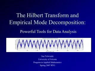
Characterization of Hall Effect Thruster Plasma Oscillations based on the Hilbert-Huang Transform. Gérard BONHOMME. and Collaborators:. Cédric Enjolras, LPMIA, UMR 7040 CNRS - Université Henri Poincaré, Nancy

E N D
Characterization of Hall Effect Thruster PlasmaOscillations based on the Hilbert-Huang Transform Gérard BONHOMME and Collaborators: Cédric Enjolras, LPMIA, UMR 7040 CNRS - Université Henri Poincaré, Nancy Stéphane Mazouffre, Luc Albarède, Alexey Lazurenko, and Michel Dudeck, Equipe PIVOINE, Laboratoire d’Aérothermique, UPR 9020 CNRS-Université d’Orléans Jacek Kurzyna, IPPT-PAN, Varsovie
Outline • Introduction • Plasma thruster oscillations • Signal processing • Experimental set-up • The EMD or Hilbert-Huang Transform • Hilbert transform and instantaneous frequency • EMD or Decomposition into Intrinsic Mode Functions (IMF) • Hilbert spectra • Analysis of SPT-100 plasma fluctuations • Filtering of different frequency ranges • Time-frequency analysis • Investigating poloidal propagation of HF oscillations • Perspectives
Hall thrusters plasma oscillationsvery large frequency range, many physical mechanisms How can we extract reliable informations from time series ? Introduction Pivoine data Non stationarity, non linearity "Classical“ Methods (Statistical Analysis, Fourier methods) drawbacks of
Short-time (or windowed) Fourier transform (DFT of sub-series) Pb : frequency resolution = 1/T the time resolution is the same at all frequencies • Wavelet tranform = generalization of the Fourier analysis change for an other analysis function giving a time resolution depending on the frequency find an orthogonal basis localised in time and frequency Solutions : Wavelets?
Principle of the wavelet transform: replace the sine waves of the Fourier decomposition by orthogonal basis functions localised in time and frequency • Aim : Decomposition of a signal into components (small waves, i.e. wavelets) corresponding to : scales or levels (i.e., frequencies) and localisations for each of these scales Two different approaches : • Continuous Wavelet Transform (e.g. Morlet) time-frequency analysis • Discrete Wavelet Transform orthogonal decomposition (filtering) Wavelet Analysis
Daubechies wavelets Analysis Discrete wavelets: Analysis and reconstruction Efficient algorithmn, But: - physical meaning of the filtering? - not well suited to time frequency analysis Synthesis
Continuous wavelets: Time-frequency analysis Fourier spectrum Pivoine data (from A. Lazurenko) Time-frequency representation obtained with Morlet wavelets Drawback cpu time demanding (because high level of redundancy)
The Hilbert-Huang Transform or Empirical Mode Decomposition Decomposition of a non stationary time-series into a finite sum of orthogonal eigenmodes, or Intrinsic Mode Functions (IMF). Self adapative approach in which the eigenmodes are derived from the specific temporal behaviour of the signal. Subsequently, the Hilbert Transform can be used to compute the instantaneous frequency and a time-frequency representation of each mode as well as a global marginal Hilbert energy spectrum. N. E. Huang et al., The Empirical Mode Decomposition and Hilbert Spectrum for Nonlinear and Non-Stationary Time Series Analysis, Proc. R. Soc. London, Ser. A, 454, pp. 903-995(1998). T. Schlurmann, Spectral Analysis of Nonlinear Water Waves based on the Hilbert-Huang transformation, Transactions of the ASME Vol.124 (2002) 22. J. Terradas et al, The Astrophys. Journal 614 (2004) 435. P. Flandrin, G. Rilling, P. Gonçalves, Empirical Mode Decomposition as a Filter Bank, IEEE Sig. Proc. Lett., Vol.11, N°2, pp. 112-114 (2004).
Hilbert transform of a data series x(t)is defined by: Hilbert Transform and instantaneous frequency By substituting we can define z(t) as the analytical signal of x(t) But in most cases the instantaneous frequency has no physical meaning from Huang et al Example • Empirical Mode Decomposition set of IMF : (1) equal number of extrema and zero crossings; (2) mean value of the minima and maxima envelopes = 0
The Empirical Mode Decomposition (sifting process) 1. Initialize : r0(t) = X(t), j=1 2. Extract the j-th IMF: a) Initialize h0(t) = rj(t), k=1 b) Locate local maxima and minima of hk-1(t) c) Cubic spline interpolation to define upper and lower envelope ofhk-1(t) d) Calculate mean mk-1(t) from upper and lower enve- lope of hk-1(t) e) Define hk(t) = hk-1(t) - mk-1(t) f) If stopping criteria are satisfied then imfj(t) = hk(t) else go to 2(b) with k=k+1 3. Define rj(t) = rj-1(t) - imfj(t) 4. If rj(t) still has at least two extrema then go to 2(a) with j=j+1, else the EMD is finished 5. rj(t) is the residue of x(t) IMF = Intrinsic Mode Functions from Huang et al A typical IMF
Analysis and Reconstruction (PIVOINE data) Analysis Synthesis
After having obtained the IMF, generated the Hilbert transform of each IMF, x(t) is represented by: This time-frequency distribution of the amplitude is designated as the Hilbert spectrum The Hilbert spectrum Two possible representations: global (as for wavelets) or for each IMF Integration in the time domain Hilbert marginal spectrum (to be compared to Fourier spectrum
The Hilbert transform compared to the continuous wavelet transform (Morlet) Example
Experimental set-up Laboratory version of a SPT 100 Hall effect Thruster Operating conditions: Ud=300 volts, Id=4.2 A Xe 5.42 mg/s Diagnostics: - Langmuir probes A7 and A8 location: thruster exit plane coaxial, unbiased, 2π/3 angular separation, 1MΩ load (Vfloat fluct.) - Current probe Acquisition: 1GHz bandwidth digital scope 250 Msamples/s, time series 50 ksamples
Results of the EMD HF bursts: 6 – 22 MHz Strongly correlated with low frequency oscillations Evidences of osc. in the Ion transit time inst. freq. domain Breathing oscillations: ~ 25 kHz Empirical Mode Decomposition of time-series from probe A7
Hilbert spectra Low frequency oscillations: • breathing mode (top) • bursts in the ion transit time frequency range HF bursts : ~ 6 – 11 –22 MHz HF bursts start mainly on a negative slope of Id with maximum amplitude ~ inflexion point minimum of Vfl and maxima of ne and Ez(A. Lazurenko)
Comparison with wavelet time-frequency analysis Morlet freq. = 375/scale 33 11.4 MHz
Because of the strong nonlinearity of HF oscillations the Fourier spectrum exhibits many peaks All these peaks do not correspond to actual modes Marginal Hilbert spectrum vs Fourier spectrum A peak in the marginal Hilbert spectrum corresponds to a whole oscillation around zero
Filtering before cross-correlating A1 A3 A6 Pivoine data from probes A1, A3, and A6(from A. Lazurenko)
probe A7 Cross-correlation functions for the HF components probe A8 HF oscillations propagate azimuthally at EB velocity v~2106 m/s Frequency peaks ~6-11-22 MHz correspond to azimuthal wavenumber m =1,2,4 A (non explained) discrepancy is observed between the phase shift measured for 120° angular separation and the period non purely azimuthal waves? Asymetry?
probe A7 probe A8 Morlet Time-frequency analysis after EMD filtering
Conclusions and Perspectives • The Hilbert-Huang Transform method: • Has proven to be a promising and attractive method to analyze non stationary and nonlinear time-series because of: - a very efficient ability in filtering different physical phenomena - accurate time-frequency representation - moderate cpu time consumption and ability to analyse long time series • Some improvements would be useful, e.g., Hilbert spectra representation • Application to Hall thruster plasma oscillations: • Clear separation of three typical time and physical scales (~25 kHz, 100-500 kHz, and ~10MHz) - unambiguous identification of bursts in the transit time inst. freq. range - analysis of HF bursts azimuthal propagation and correlation with Id • More reliable experimental data are needed to go further into the physics of the observed plasma fluctuations, in particular to get an accurate access to azimuthal and axial propagation. (J. Kurzyna et al., submitted to PoP)
with =10 ; =2. ; f0=1 Fourier transform definition • F () complex lnformation on time localisation contained in the phase difficult access • Example 1 A musician playing either successively two notes, or simultaneously these two notes same amplitude spectra Drawbacks of Fourier methods Spectral density chirp with = 1. ; 0 =10
Principle : mother-wavelet (t) Translation + dilatation The Continuous Wavelet Transform Wavelet Transform normalisation compact support orthogonal basis in L2(R) Pb : find a "good " mother-wavelet Necessary conditions (admissibility) : (reconstruction) Parseval’s theorem Morlet wavelets with with: Time resolution Frequency resolution (with )
d = 1 Morlet Wavelet Mother-wavelet k=2, t0=0, T=1 Maximum at T = k Morlet transform: convolution product f*T with
Drawbacks of the continuous wavelet transform :redondancy, CPU time, admissibility conditions non completely fullfilled (Morlet) The Discrete Wavelet Transform Solution ?Discrete Wavelets(similar to the DFT) • Octave scaling Tj = 2j et t0 j,k = k/ 2j • orthogonality with There are 2m base functions at the m level • reconstruction from Newland [1]
Haar lack of regularity • Daubechies wavelets - must be determined by recurrence from a scaling function (t) (Meyer, 1993) - they are completely defined by the coefficients ck 2r+1 conditions must be satisfied: Wavelet construction: Daubechies wavelet (t) for r=2 (from Newland [1])
Solutions : • Haar (r=1) c0 = c1 = 1 • Daubechies D4 (r=2) • r > 3, (numerical computation) discrete transform (computed by using the Mallat algorithm) analysis, and reconstruction formula synthesis Mallat tree (pyramid algorithm) D4 D20 from Newland [1]
The Continuous Wavelet Transform (Morlet): FFT computation of Practically f={fn} et N=2m • Oversampling of F() required solution = zero padding of fn (for T=NTe (N-1)N zeros) Practical considerations (1) See for example, D. Jordan et al, Rev.Sci.Instrum. 68 (1997) 1484-1494
Discrete Wavelet Transform: pyramid algorithm (no need for theW(t)) ½L3 ½ H2 ½ H1 example : f=f(1:8) ——— f'(1:4) ——— f'(1:2) ——— f'(1) ½ H3 ½ H2 ½ H1 a[5:8] a[3:4] a(2) a(1) Hn et Ln are matrices build directly from the ck coefficients (cf. Newland [1]) Practical considerations (2) Low-pass filter High-pass filter
Analysisand reconstruction of asquare wave Analysis Synthesis
pulse = 10 ; = 0.5 ; f0 = 0.5 = 0.1 ; = 1. ; 0 = 10 chirp Time-frequency analysis
The completeness is established both theoretically and numerically Completeness and Orthogonality The orthogonality is satised in all practical sense, but it is not guaranteed theoretically IO = overall index of orthogonallity for this example IO = 0.0067 or for two IMF: Example (from Huang [1])
The degree of stationarity DS is defined as: Degree of stationarity with mean marginal spectrum and the degree of statistic stationarity DSS can be is defined as: If the Hilbert spectrum depends on time, the index will not be zero, then the Fourier spectrum will cease to make physical sense. The higher the index value, the more non-stationary is the process.
IMF 1-4 Application to experimental time-series (PIVOINE) Signal analysé Spectre de Hilbert marginal J. Kurzyna et al., submitted to Phys. of Plasmas IMF 9