CLIC
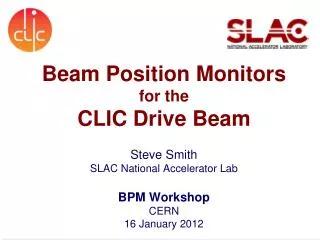
Beam Position Monitors for the CLIC Drive Beam Steve Smith SLAC National Accelerator Lab BPM Workshop CERN 16 January 2012. CLIC. Linear Collider Two-Beam acceleration Accelerate Drive beam high current (100Amp) low energy (1GeV) long pulse (140 microsec ). Extract RF from drive beam

CLIC
E N D
Presentation Transcript
Beam Position Monitorsfor the CLIC Drive Beam Steve SmithSLAC National Accelerator LabBPM WorkshopCERN16 January 2012
CLIC • Linear Collider • Two-Beam acceleration • Accelerate Drive beam • high current (100Amp) • low energy (1GeV) • long pulse (140 microsec) • Extract RF from drive beam • Transfer to luminosity beam • Lower current (1 A) • High energy (1.5 TeV) • Short pulse ( 150 ns)
Beam Position Monitors • Main Beam • Quantity ~7500 • Including: • 4196 Main beam linac • 50 nm resolution • 1200 in Damping & Pre-Damping Ring • Drive Beam • Quantity ~45000 • 660 in drive beam linacs • 2792 in transfer lines and turnarounds • 41000 in drive beam decelerators • !
CLIC Drive Beam Decelerator BPMs • Requirements • Transverse resolution < 2 microns • Temporal resolution < 10 ns Bandwidth > 20 MHz • Accuracy < 20 microns • Wakefields must be low • Considered Pickups: • Resonant cavities • Striplines • Buttons
Drive Beam Decelerator BPM Challenges • Bunch frequency in beam: 12 GHz • Lowest frequency intentionally present in beam spectrum • It is above waveguide propagation cutoff • TE11 ~ 7.6 GHz for 23 mm aperture • There are non-local beam signals above waveguide cutoff. • Example of non-local signal: • Structure purpose is to generate 130 MW @ 12 GHz in nearby Power Extraction Structures (PETS) • Leakage to BPM? • Also transverse modes induced by • Aperture asymmetries • beam offsets
Generic Stripline BPM • Algorithm: • Measure amplitudes on 4 strips • Resolution: • Small difference in big numbers • Calibration is crucial! Given: R = 11.5 mm and sy < 2 mm Requires sV/Vpeak = 1/6000 12 effective bits
Choose Operating Frequency • Operate at sub-harmonic of bunch spacing ? • Example: FBPM = 2 GHz • Signal is sufficient • Especially at harmonics of drive beam linac RF • Could use • buttons • compact striplines • But there exist confounding signals • OR process at baseband ? • Bandwidth ~ 4 - 40 MHz • traditional • resolution is adequate • Check temporal resolution • Requires striplines to get adequate S/N at low frequencies (< 10 MHz) Transverse errors at frequency of bunch combination ! ! ! OK
Decelerator Stripline BPM Diameter: 23 mm Stripline length: 25 mm Width: 12.5% of circumference (per strip) Impedance: 50 Ohm striplines Quad
Signal Processing Scheme • Lowpass filter to ~ 40 MHz • Digitize with fast ADC • 160 Msample/sec • 16 bits, 12 effective bits • Assume noise figure ≤10 dB Including Cable & filter losses amplifier noise figure ADC noise • For nominal single bunch charge 8.3 nC • Single bunch resolution y < 1 mm
Single Bunch and Train Transient Repsonse • What about the turn-on / turn-off transients of the nominal fill pattern? • Provides good position measurement for head/tail of train • Example: NLCTA • ~100 ns X-band pulse • BPM measured head & tail position with 5 - 50 MHz bandwidth • CLIC Decelerator BPM: • Single Bunch Full Train • Q=8.3 nC I = 100 Amp • y ~ 2 mm y < 1 mm (train of at least 4 bunches)
Temporal Response within Train • Simulate 10 MHz transverse oscillation at 2 micron amplitude • Up-Down stripline difference signal • S/Nthermal is huge • BUT the ADC noise limit: ~ 2 m/Nsample
Craft Bandwidth • Maintain adequate S/N across required spectrum • In presence of linearly rising signal vs. frequency • Aim for roughly flat S/N vs. frequency from few MHz to 20 MHz • Choose two single-pole low-pass filters plus one 2nd order lowpass • Look at spectrum while manually tweaking poles. • Example: • F1 = 4 MHz • F2 = 20 MHz • F3 = 35 MHz
Origin of Position Signal • Convolute pickup source term • for up/down electrodes • to first order in position y • With stripline response function • where Z is impedance and • l is the length of strip • At low frequency << c/2L ~ 6GHz • Looks like derivative: Up-Down Difference: • 1st term: Y dQ/dt • 2nd term: dY/dt Q • Signal is nice, but is a product of functions of time, and their derivatives. Can predict waveform from y(t) and Q(t) • But how about inverse? Nonlinear ! Inconvenient !
Position & Charge • Back up one step: • At low frequency << c/2L ~ 6GHz • Looks like derivative: • Take sum and difference: Sum & Difference • The expression for is linear in Q(t) • Can estimate from digitized waveforms with standard tools • Deconvolution • If we know response function • Measure impulse response function with a single bunch • or a few bunches • e.g. < few ns of bunch train • Then having solved for Q(t) • insert Q(t) in expression for and solve for y(t)
Assumptions • ADC • Sampling rate = 200 MHz • S/N = 77 dBFS • Record length = 256 samples • Assume excellent linearity • ADC has excellent linearity • Don’t mess up linearity in the amplifiers! • Specify high IP3 for good linearity • Zeven = Zodd • Even / odd mode impedances are equal • probably not important assumption • the difference can be estimated in 2D EM solver • To be investigated
Algorithm • Define frequency range of interest • 0.5 MHz < f < 40 MHz • Acquire single bunch data • Invert single bunch spectrum • Roll off < 0.5 MHz and > 40 MHz • (maintaining phase info) • Acquire bunch train data • Form D & S • Deconvolute with impulse response from single bunch acquisition • Divide Fourier Transform of data by (weighted) FT of single bunch
Example • Simulate Bunch train with position variation • Simulate response • Form D and S (difference & sum) • Deconvolute • Compare to generated y(t)
Charge & Position vs. Time • Works quite well • On paper • Must add effects of nonlinearities • Can deconvolute Q(t) and y(t) from sum and differences of digitized stripline waveforms • Dynamic range of ADC makes it challenging
Summary of Performance • Single Bunch • For nominal bunch charge Q=8.3 nC • y ~ 2 mm • Train-end transients • For current I = 100 Amp y < 1 mm (train of at least 4 bunches) • For full 240 ns train length • current I > 1 Amp • resolution y < 1 mm • Within train • For nominal beam current ~ 100 A sy ~ 2 mm for t > 20 ns
Calibration Calibrate Y Calibrate X • Transmit calibration from one strip • Measure ratio of couplings on adjacent striplines • Repeat on other axis • Gain ratio BPM Offset • Repeat between accelerator pulses • Transparent to operations • Extremely successful at LCLS (SLAC)
Finite-Element Calculation • Characterize beam-BPM interaction • GDFIDL • Thanks to Igor Syratchev • Geometry from BPM design files • Goals: • Check calculations where we have analytic approximations • Signal • Wakes • Look for • trapped modes • Mode purity Port Signal Transverse Wake
Transverse Wake • Find unpleasant trapped mode near 12 GHz (!) • Add damping material around shorted end of stripline • Results: • Mode damped • Response essentially unchanged at signal frequency Transverse Wake
Damped Stripline BPM • Few mm thick ring of SiC • Transverse mode fixed • Signal not affected materially • Slight frequency shift Damping Material Wake __ Damped __ Undamped Signal Transverse Impedance Signal Spectrum
Comparison to GDFIDL • Compare to analytical calculation of “perfect stripline” • Find resonant frequencies don’t match • GDFIDL ~ 2.3 GHz • Analytic model is 3 GHz • Is this due to dielectric loading due to absorber material? • Amplitudes in 100 MHz around 2 GHZ differ by only ~5% (!) • Energy integrated over 1 bunch: • 0.16 fJ GDFIDL • 0.15 fJMathcad • Must be some luck here • filter functions are different • resonance frequencies don’t match • Effects of dielectric loading partially cancels • Lowers frequency of peak response raises signal below peak • Reduces Z decreases signal
Sensitivity • Ratio of Dipole to Monopole • D/S ratio • GDFIDL calculation • Signal in 100 MHz bandwidth around 2 GHz • Monopole 1.75 mV/pC • Dipole 0.25 mV/pC/mm • Ratio 0.147/mm • Theory • y = R/2*D/S • Ratio of dipole/monople = 2/R = 0.148/mm for R =13.5 mm • (R of center of stripline, it’s not clear exactly which R to use here) • Excellent agreement for transverse scale
Multibunch Transverse Wake • Calculate transverse wakefield: • GDFIDL shows quasi-DC Component: 30.6 mV/pC/mm/BPM • Calculate 27 mV/pC/mm/BPM for ideal stripline • Excellent agreement • Components at 12 GHz, 24 GHz, 36 GHz: • Comparable to features of PETS • Compare with GDFIDL:
Longitudinal Wakefrom GDFIDL Multibunch: • No coherent buildup • Peak voltage unchanged • Multiply by bunch charge in pC to get wake • 8.3 nC/bunch Single Bunch
Summary of Comparison to GDFIDL • GDFIDL and analytic calculation agree very well on characteristics • Signals at ports: • Monopole • Dipole • Transverse Wake • Disagreement on response null at signal port • May need lowpass filter to reduce 12 GHz before cables • Signal Characteristics Good • Longitudinal & transverse wakes are OK
Summary • A conventional stripline BPM should satisfy requirements • Processing baseband (4 – 40 MHz) stripline signals • Signals are local (not subject to modes propagating from elsewhere) • Calculation agrees with simulation: • Wakefields • Trapped modes • Should achieve required resolution • Calibrate carefully • Online • transparently • Should have accuracy of typical BPM of this diameter • Pay attention to source of BPM signal • Need to unfold position signal y(t) • Must occasionally measure response function • with single bunch or few bunch beam Conventional, well-established Novel, untested