8. Numerical methods for reliability computations
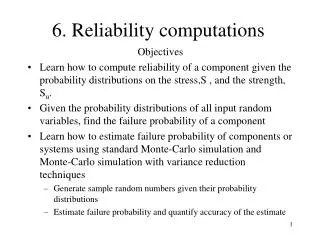
8. Numerical methods for reliability computations. Objectives Learn how to approximate failure probability using Level I, Level II and Level III methods. Level I, II, III methods. Crude, economical. Level I methods: use one parameter to account for the uncertainty in each random variable


8. Numerical methods for reliability computations
E N D
Presentation Transcript
8. Numerical methods for reliability computations Objectives • Learn how to approximate failure probability using Level I, Level II and Level III methods
Level I, II, III methods Crude, economical • Level I methods: use one parameter to account for the uncertainty in each random variable • Level II methods: use two parameters to account for the uncertainty in each random variable (usually the mean and the standard deviation) • Level III methods: take into account for the probability distributions of the random variables. More accurate, But also more expensive
First order, second moment methods • Reduced random variables. Independent, standard normal variables obtained from a transformation of random variables. • Safety index, =distance from straight line representing the boundary between survival and failure and origin in space of reduced variables. Failure probability=(- ). • Of all combinations of the r.v. that entail failure the one corresponding to the most probable failure point is the most likely.
OA=safety index OB=safety index if X1 were deterministic OC=safety index if X2 were deterministic X2 more important than X1 z2 Constant joint probability density C O z1 A, most probable failure point B
Lessons learnt (refer to the previous slide) • If performance function is linear, it is easy to compute the failure probability exactly. • If we plot the limit state function in the space of the random variables, then this function is represented by a straight line. • The safety index, , is equal to the distance of the straight line representing the limit state function to the origin. The probability of failure is (-). • Of all combinations of values of the values of the random variables, the one corresponding to the most probable failure point, A, is the most likely
Finding the most probable point when the performance function is linear and the random variables are independent, standard normal g(z1,z2 )=a0+a1z1+a2z2 z2 z*1, z*2 g<0 gradient of g g>0 O z1
Estimating failure probability using linear approximation of the performance function about MPP: First order methods (FORM) or First order, second moment methods (FOSM) • It is important to approximate g-function accurately in the vicinity of MPP to estimate failure probability accurately. Therefore, we should use linear Taylor expansion about the MPP. • Case A: standard normal, independent random variables • Case B: correlated standard normal random variables • Case C: independent variables with arbitrary probability distributions • Case D: dependent variables with arbitrary probability distributions (beyond the scope of this class)
Case A: normal independent random variables Transform variables into standard normal Find MPP: Find z1*,…,zn* To minimize (z1*2+…+zn*2)1/2 So that g(z1*,…,zn*)=0 Find safety index, and P(F)
Performance function in the space of reduced random variables Linear approximation of limit state function, g(z)=0 Limit state function,g(z)=0 z2 MPP: z1*, z2* Gradient of g Failure region O z1 Safe region
Case B Correlated, standard normal random variables • Need to transform correlated variables into uncorrelated • Transformation: rotation of coordinate system • Y=TTX • T: matrix whose columns are the eigenvectors of the covariance matrix
Case C:Independent random variables with arbitrary probability distribution • Transform random variables to standard normal using Rosemblatt transformation (the same transformation is used for generating random variables with arbitrary probability distributions) z x x, z
Reliability computations: practical considerations • Available methods: FORM, Monte Carlo, direct integration of PDF • FORM: can be tricky but it can be the only feasible approach for many complex problems • Validate the results using Monte-Carlo for in a few cases • Conduct parametric studies to understand what the important variables are • Understand the behavior of the performance function • Remove the unimportant random variables and repeat the analysis to see if the results change • Repeat the procedure for finding MPP starting from different initial points to see if there are multiple MPPs
Suggested reading • Der Kiureghian, “First- and Second-Order Reliability Methods,” Engineering Design Reliability Handbook, CRC press, 2004, p. 14-1. • Thoft-Christensen, “System Reliability,” Engineering Design Reliability Handbook, CRC press, 2004, p. 15-1.